Measuring cloud optical depth with a balloonborne microlidar operated from the stratosphere

The Balloonborne Cloud Observing micrOLidar (BeCOOL) has been developed to be operated onboard a stratospheric balloon in order to monitor the atmosphere below 20 km, more particularly thin ice clouds. This backscatter lidar operating at 802 nm was designed to maintain a high level of performance while keeping its mass below 6 kg and limiting its power consumption to 4 W on average. Several balloons embarking BeCOOL instruments have been launched from the Tropics (Seychelles Islands, −4.68° S +55.45° E) during the Stratéole2 campaign organized by the French Space Agency (Centre National d'Etudes Spatiales, CNES) in autumn and winter 2021–2022. The microlidar system, its operational performances, and the data processing to estimate optical properties are described. BeCOOL is able to measure optical depth of upper level thin ice clouds down to $\mathrm{2}\times {\mathrm{10}}^{-\mathrm{5}}$. It is possible to constrain the lidar ratio when the cloud optical depth is larger than $\mathrm{3}\times {\mathrm{10}}^{-\mathrm{2}}$. In this case, the optical depth relative uncertainty is less than 5 %.

1 Introduction

Lidar technique is powerful to monitor cloud properties in the atmosphere from a large variety of platforms. Large systems can be easily used to perform cloud observations from the ground, but low-level cloud coverage make it difficult to observe continuously high level clouds. Operating from space or from a high altitude airborne platform, such as a stratospheric balloon, is better suited to study the properties and life-cycle of elevated thin cirrus. The Balloonborne Cloud Observing micrOLidar (BeCOOL) system was designed to be implemented onboard stratospheric pressurized balloons (SPBs) operated by the French Space Agency (Centre National d'Etudes Spatiales, CNES) during the Stratéole2 campaign (Haase, 2018).

This observation campaign focuses on the Tropical Tropopause Layer (TTL, Fueglistaler et al., 2009), a region of the climate system where the coupling between dynamical, radiative, and microphysical processes has global impacts. In particular, thin cirrus clouds in the TTL play a critical role in Earth’s radiative budget and regulate the amount of water vapor entering the stratosphere, directly influencing global climate (Randel and Jensen, 2013). Their widespread but optically subtle presence makes them a major source of uncertainty in climate models, as they modify local radiative fluxes and affect the thermal structure of the tropical tropopause. The long-duration Stratéole2 balloons, drifting for weeks just above the TTL, provide an ideal platform for observations with BeCOOL. With this elastic backscatter lidar it is possible to measure the cirrus optical thickness at one wavelength, and to characterize the spatial variability and lifetime of these clouds (Lesigne et al., 2024, 2025).

The first stratospheric balloon-borne lidar observations were achieved during the HIBISCUS campaign with the Microjoule Lidar (MULID) system, providing nighttime measurements of tropical cirrus clouds (Pommereau et al., 2011; Di Donfrancesco et al., 2006). Later, the Balloon Lidar Experiment (BOLIDE) system (Kaifler et al., 2020) demonstrated the feasibility of high-power lidar systems on balloon platforms, observing polar mesospheric clouds during a 6-d flight at ∼38 km altitude, with payloads and power requirements adapted to larger platforms. Operating a lidar onboard a small gondola implies strong constrains in terms of available space and energy. For SPB-compatible systems, the BeCOOL approach aligns with the microlidar philosophy of MULID. A more efficient emitting laser diode source was used for BeCOOL, and the optical design took advantage of fibered optical transfer between the main optics and the emission/reception lenses. This provides better temperature isolation and a higher signal-to-noise ratio (SNR) during nighttime measurements. The design of BeCOOL also benefited from developments of autonomous microlidar systems for Arctic operations within the Ice Atmosphere Arctic Ocean Observing System (IAOOS) project (Mariage et al., 2017; Maillard et al., 2021).

The nadir-pointing microlidar observations are geometrically comparable to spaceborne lidar measurements. The Cloud-Aerosol Lidar with Orthogonal Polarisation (CALIOP, Winker et al., 2009, 2010), onboard the Cloud Aerosol Lidar and Infrared Pathfinder Satellite Observations (CALIPSO), was still operating during the 2021–2022 Stratéole2 winter campaign. As detailed later, the processing of BeCOOL measurements partly relies on these reference observations.

BeCOOL system and its operation in the stratosphere is described in Sect. 2. The retrieval of the attenuated backscatter profile, including the choice of an overlap function and procedure to normalize the signal, is detailed in Sect. 3. The inversion procedure to compute the backscatter profile and cloud optical depths, including the issue of multiple scattering, is described in Sect. 4. The estimate of the uncertainty of the cloud optical depth is given in Sect. 5. Conclusions and perspectives are drawn in Sect. 6, either in terms of scientific questions or campaigns that can be addresses by operating BeCOOL, or of future technical improvement to overcome the current limitation of this microlidar.

2 Instrument description and operation

2.1 Operating a microlidar from the stratosphere

BeCOOL is embedded inside Zephyr gondola, a platform designed by the CNRS DT-INSU. This platform drifts at an atmospheric pressure level of 50 hPa (altitude of about 20 km in the Tropics) below a stratospheric pressurized balloon operated by CNES. It is supposed to fly up to 3 months. For safety reason the Zephyr gondola is constrained to be small and light (less than 1 m high and about 0.6 m wide). This drastically limits the mass and the volume of the microlidar. Inside the gondola, room is left for other instruments and for the Zephyr OnBoard Computer (OBC) in charge of communications with the ground and of the management of the full payload. The Zephyr gondola is equipped with solar panels recharging embedded batteries. Zephyr provides power continuously, for a total average power lower than 25 W. Regular Iridium communications make it possible to receive telecommand and to send the data.

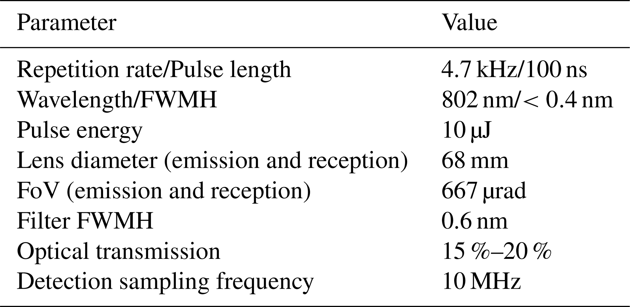
Operating from the stratosphere prevents the microlidar from any icing or condensation issues on optics, but the low atmospheric pressure make it difficult to obtain an efficient thermal regulation for components requiring it for optimal efficiency. Taking into account all these constrains drove the design of BeCOOL and led to the block diagram shown in Fig. 1. This microlidar is composed of three main subsystems: the optical head (OH, microlidar lenses), the optical box (OB) and the electronic box (EB). The total weight of BeCOOL is less than 6 kg and is roughly split between OH (3 kg), EB (1 kg) and OB (1.8 kg). To perform nadir measurements a specific aperture was made in a separate lower part of the gondola where the lenses are located. This arrangement is possible thanks to the use of optical fibers. This way, the thermal sensitive parts of the microlidar (laser diode, optical filter) are located in a more insulated upper part of the gondola as shown in Fig. 2. BeCOOL main features values are shown in Table 1.

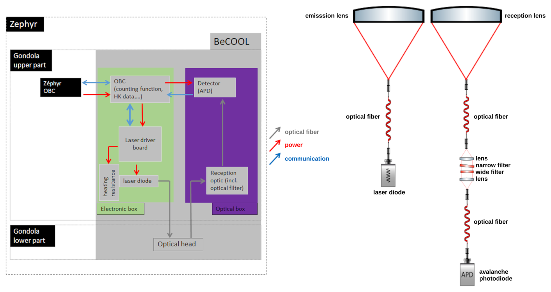
Figure 1 Left: BeCOOL block diagram. The green area corresponds to the electronic box. It includes the on-board computer (OBC) of the lidar. The purple area corresponds to the optical box (OB). It includes the avalanche photodiode (APD). The optical head includes the emission lens and the reception lens. Right: Optic schematic drawing showing both emission (left) and reception (right) channel .

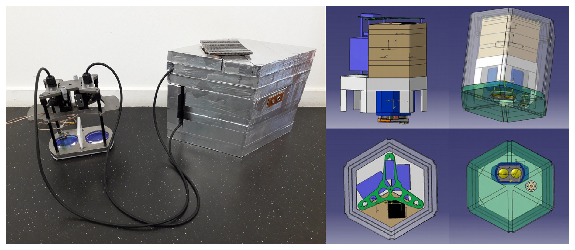
Figure 2 Picture (left) and 3D drawing (right) of BeCOOL microlidar. The optical head (OH) equipped with two lenses can be seen in the lower (“cold”) part of the gondola. The two other boxes with diamond shape are shown in brown in the upper (“hot”) part of the gondola, sharing the volume with the Zephyr electronic, other instruments and the batteries.

Table 1 Main characteristics of BeCOOL. FWHM is the Full Width at Mid Heigth. FoV is the Field of View.

2.2 Emission channel

The laser source is located in the EB. It is a compact and spectrally narrow (<0.4 nm) laser diode module emitting around 802 nm provided by DILAS. It is optically fibered (105 µm; NA 0.22) and linked to the OH at the emission lens focal point, so that the emission divergence is about 660 µrad. This laser module is powered by a laser driver board (LDB) designed and provided by the French company CIMEL Electronique to obtain a pulsed emission at a frequency of about 4.7 kHz with pulse energy of about 10 µJ. The LDB receives commands from the BeCOOL OBC to start or stop the laser emission, and sends housekeeping data such as temperatures (including laser diode temperature), voltage and current, as well as synchronization signal to synchronize emission and photon counting electronics. The LDB is also in charge of the laser diode thermal regulation via a heating resistance since the emitted spectrum is sensitive to thermal variation. A shift in temperature may impact the microlidar global efficiency. Indeed, the emission wavelength must stay within the spectral window of the optical filter of the reception channel.

2.3 Reception channel

The backscattered signal is collected by the OH where an optical fiber (105 µm; NA 0.22) is located at the reception lens focal point. This optical fiber links the OH to the filtering optic located in the OB, where two interferential filters reject the background signal from the sky. The spectral width of the interferential filter is larger than the emitted spectrum. This prevents the overall optical transmission from dropping because of a too important thermal shift impacting either the laser diode or the interferential filter. The APD is linked to the output of the filtering optic by an optical fiber with the same characteristic. Each photon detected by the APD produces an electronic pulse which is then accumulated by the OBC to obtain an atmospheric profile of backscattered signal with a 15-m spatial resolution up to 21.2 km below the microlidar. The highest time resolution of BeCOOL is about 1 s. Iridium communications used to recover the atmospheric profiles on ground are not efficient enough to transfer continuous measurements with such a resolution. The time resolution has been decreased by averaging 60 highly resolved atmospheric profiles. When operated onboard Zephyr, the ultimate time resolution of BeCOOL is therefore about 1 min. During the campaign, in order to prevent overheating of the laser diode (lack of convection prevents from using active cooling with a Peltier module), BeCOOL only measuring half of the time during a duty cycle (10 min ON mode, to 10 min OFF). Since BeCOOL average consumption is about 8 W, with peak up to 13 with the laser heating resistance, this 50 % duty cycle led to a global in-flight consumption of 4 W.

2.4 Pre-campaign optimization of the alignment

The temperature differs significantly between the ground-based environment, where BeCOOL is mechanically assembled and aligned, and the in-flight environment. This thermal difference distorts the optomechanical structure of the OH, resulting in an in-flight misalignment between the emission and reception optical axes. To mitigate this in-flight misalignment, an empirical strategy is implemented: an “in-lab controlled misalignment” is introduced on the ground, such that BeCOOL becomes correctly aligned once it reaches its operational altitude. To determine the appropriate “in-lab controlled misalignment”, the microlidar is placed in a climatic chamber whose temperature and pressure match those expected during the campaign. Inside the chamber, BeCOOL is mounted on a thermally insensitive optical retroreflector that enables a parallel optical injection from the emission axis into the reception axis. The optical power injected into the reception fiber is used as a proxy to assess the optical alignment. The optomechanical adjusters of the microlidar are equipped with small motors whose rotation compensates for the induced optomechanical distortion. The motor rotation is monitored quantitatively in order to determine the appropriate “in-lab controlled misalignment” that will optimize the performance of BeCOOL when operated in the stratosphere.

3 Retrieval of the attenuated backscatter profile

In this section, we consider instrumental corrections and raw signal normalization to derive the attenuated backscattering profile. The inversion process to compute the backscatter profile and estimate optical depth is described in the next section.

3.1 Range corrected lidar signal

The raw signal P(t) measured by the photodiode against time is first corrected from saturation using a set of factory parameters. In most cases, this correction leads to a signal enhancement lower than 1 %, very exceptionally reaching values up to 20 % over strongly backscattering cloud tops. We note P^* the signal corrected from saturation. Looking downward, the lidar is operating in a passive mode once the ground has been hit by the laser pulse. We thus average the tail of the signal beyond this ground echo to estimate the constant background value P^*(∞) of the sky radiance measured by the lidar when operating like a radiometer. Noting r the distance between the lidar and the atmospheric layer illuminated at time t, with $r=ct/\mathrm{2}$, where c is light velocity, we estimate the range corrected lidar signal $Z\left(r\right)=\left[P^{*}\right(r)-P^{*}(\mathrm{\infty }\left)\right]r^{\mathrm{2}}$.

Given the classical lidar equation, we know that the range corrected signal is a function of atmospheric properties:

$$\begin{array}{}\text{(1)}& \begin{array}{rl}Z\left(r\right)& =K\times O\left(r\right)\left[{\mathit{\beta }}_{\mathrm{p}}\right(r)+{\mathit{\beta }}_{\mathrm{m}}(r\left)\right]\\ & \exp \left[-\mathrm{2}\underset{\mathrm{0}}{\overset{r}{\int }}\mathit{\eta }\left[{\mathit{\alpha }}_{\mathrm{p}}\right(r^{\prime })+{\mathit{\alpha }}_{\mathrm{m}}(r^{\prime }\left)\right]\mathrm{d}{r}^{\prime }\right]\\ & =K\times O\left(r\right)\mathit{\beta }\left(r\right)\left[T\right(r){]}^{\mathrm{2}}\end{array}\end{array}$$

K is the instrumental constant, O(r) the lidar overlap function, β_p(r) and β_m(r) the particular and molecular backscatter coefficients at range r, α_p(r) and α_m(r) the particular and molecular extinction coefficients at range r, and η a correction parameter accounting for multiple scattering (η=1 for single scattering). We note $\mathit{\beta }\left(r\right)={\mathit{\beta }}_{\mathrm{p}}\left(r\right)+{\mathit{\beta }}_{\mathrm{m}}\left(r\right)$ the total backscatter coefficient and $T\left(r\right)=\exp \left(-{\int }_{\mathrm{0}}^r\mathit{\eta }\left[{\mathit{\alpha }}_{\mathrm{p}}\left(r^{\prime }\right)+{\mathit{\alpha }}_{\mathrm{m}}\left(r^{\prime }\right)\right]\mathrm{d}{r}^{\prime }\right)$ the transmission of the atmosphere between the lidar and the atmospheric layer sampled at range r.

We want to estimate the attenuated backscatter coefficient B(r)=β(r)[T(r)]². According to Eq. (1), $B\left(r\right)=\frac{Z\left(r\right)}{O\left(r\right)K}$. We thus need to determine the overlap function of O(r) (Sect. 3.2) and the value of K (Sect. 3.3).

3.2 Overlap function

Even if the microlidar was optimized in a thermal chamber in order to be aligned when operated in the stratosphere, (Sect. 2.4), a misalignment of the optical axes of the emission and of the reception channels was expected in real conditions. The overlap is not only a function of the field of views of these two channels but also of the angular tilt between their optical axis. In order to understand what drives the overlap function O(r), we first computed its theoretical shape following Ancellet et al. (1986). Considering the plane defined by the optical centers of the two lenses and the direction of the two optical axes when perfectly aligned, the angular tilt can be split into two parts, one parallel to this plane, one perpendicular to this plane. Perpendicular misalignment only reduces the overall transmission of the system and has no impact on the shape of the overlap function. Figure 3a shows simulations of overlap functions for different angles of parallel misalignment, considering converging optical axes. The larger the angle, the smaller the value of overlap once an almost constant value is reached, several kilometers away from the platform. Figure 3b shows the same functions, arbitrarily normalized at a distance of 1.5 km. It emphasizes the large variability of the overlap function in the first 2 km.

These theoretical functions have been compared to empirical overlap functions. For a given instrument it is possible to compute the shape of O(r) as the ratio between the range-corrected profiles for clear sky conditions (no clouds or aerosol layers) and the average attenuated backscatter profile derived from corresponding ERA5 pressure and temperature fields (Hersbach et al., 2020), following Bucholtz (1995) to calculate Rayleigh scattering cross-sections. The black line on Fig. 3b is an example of such an empirical function, normalized 1.5 km away from the laser source. It turns out that the shape of the overlap function is mostly driven by the parallel misalignment angle between the two optical axes. The misalignment slightly evolves with the temperature of the optical head, which exhibits a diurnal cycle linked with day/night contrast that leads to a small but systematic re-alignment of the optical channels during each night. It turns out that this is a second order effect. Indeed the instrumental constant K strongly depends on the temperature (see Sect. 3.3). It is therefore difficult to disentangle the estimates of K and of O(r). This issue has been investigated. We have found that the uncertainty on the overlap function due to the alignment angle dependence on temperature is smaller than 10 %. For a given instrument we thus consider a constant overlap function over time. Following the procedure described in this section, a smoothed empirical overlap function is estimated for each instrument, making it possible to compute $Z\left(r\right)/O\left(r\right)$.

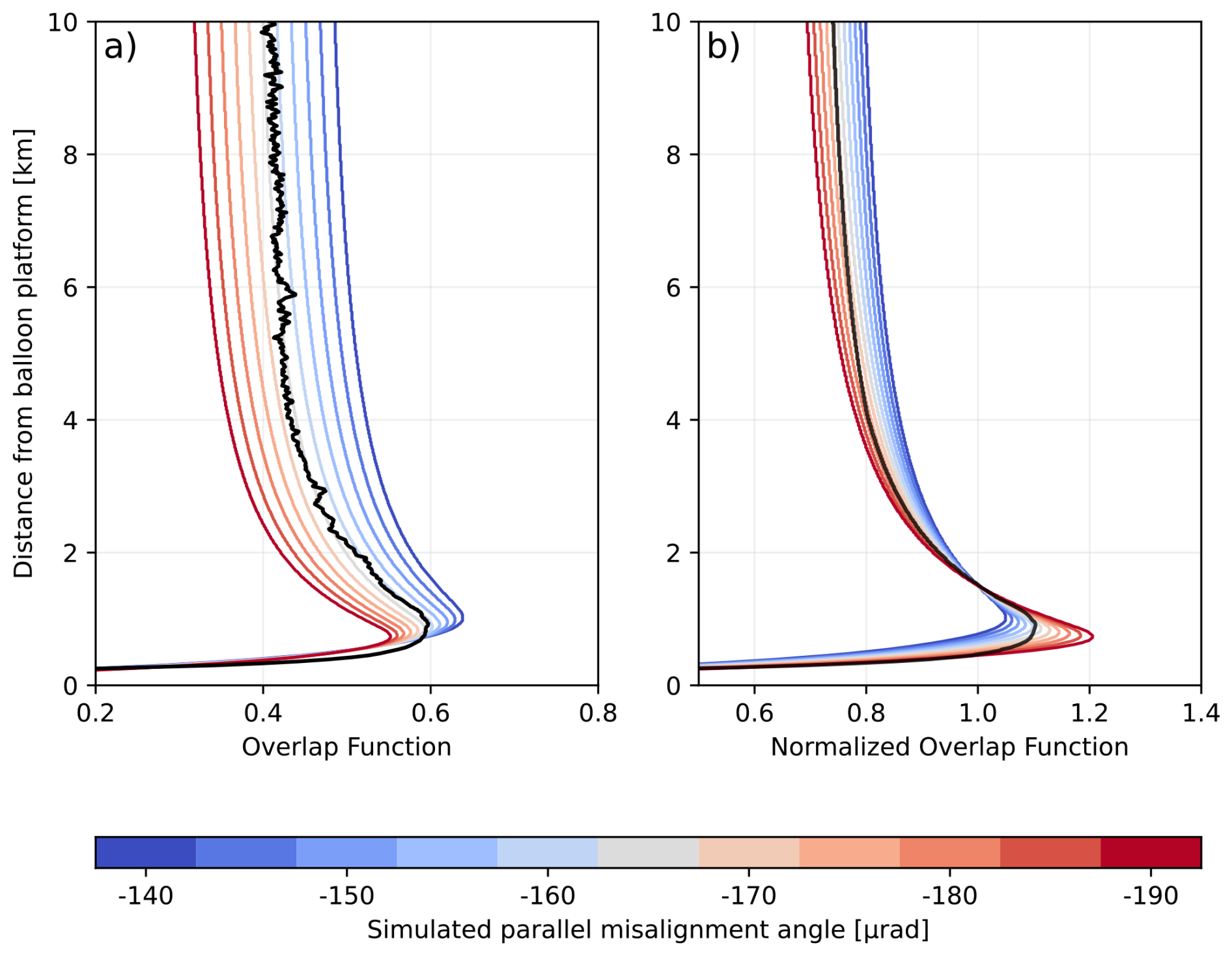
Figure 3 (a) Simulated overlap functions for different parallel misalignment angles between the emission and the reception optical channels. The parallel misalignment angle varies from −140 (blue line) to −190 µrad (red line). Negative values correspond to slightly converging optical axes. The solid black line is a reference clear sky profile used to derive the empirical overlap correction for a given instrument: it is the ratio of the mean lidar profile over a 3 h cloud-free window to a synthetic Rayleigh lidar profile. (b) Same overlap functions (blue to red lines) normalized at a distance of 1.5 km from the platform, along with the empirical overlap correction (smooth solid black line) derived from the reference clear-sky profile, normalized at the same distance.

3.3 Signal normalization

Lidar signals have now to be normalized in order to compute the attenuated backscatter profiles. Ideally, the instrumental constant K should be evaluated using a region of the atmosphere where molecular scattering is prevailing. In this region, the expected value of B(r)=β(r)[T(r)]² can be computed assuming β(r)=β_m(r). CALIOP benefits from a region of almost pure molecular atmosphere above 35 km which enables the normalization upon synthetic Rayleigh lidar profiles build from MERRA-2 reanalysis (Kar et al., 2018).

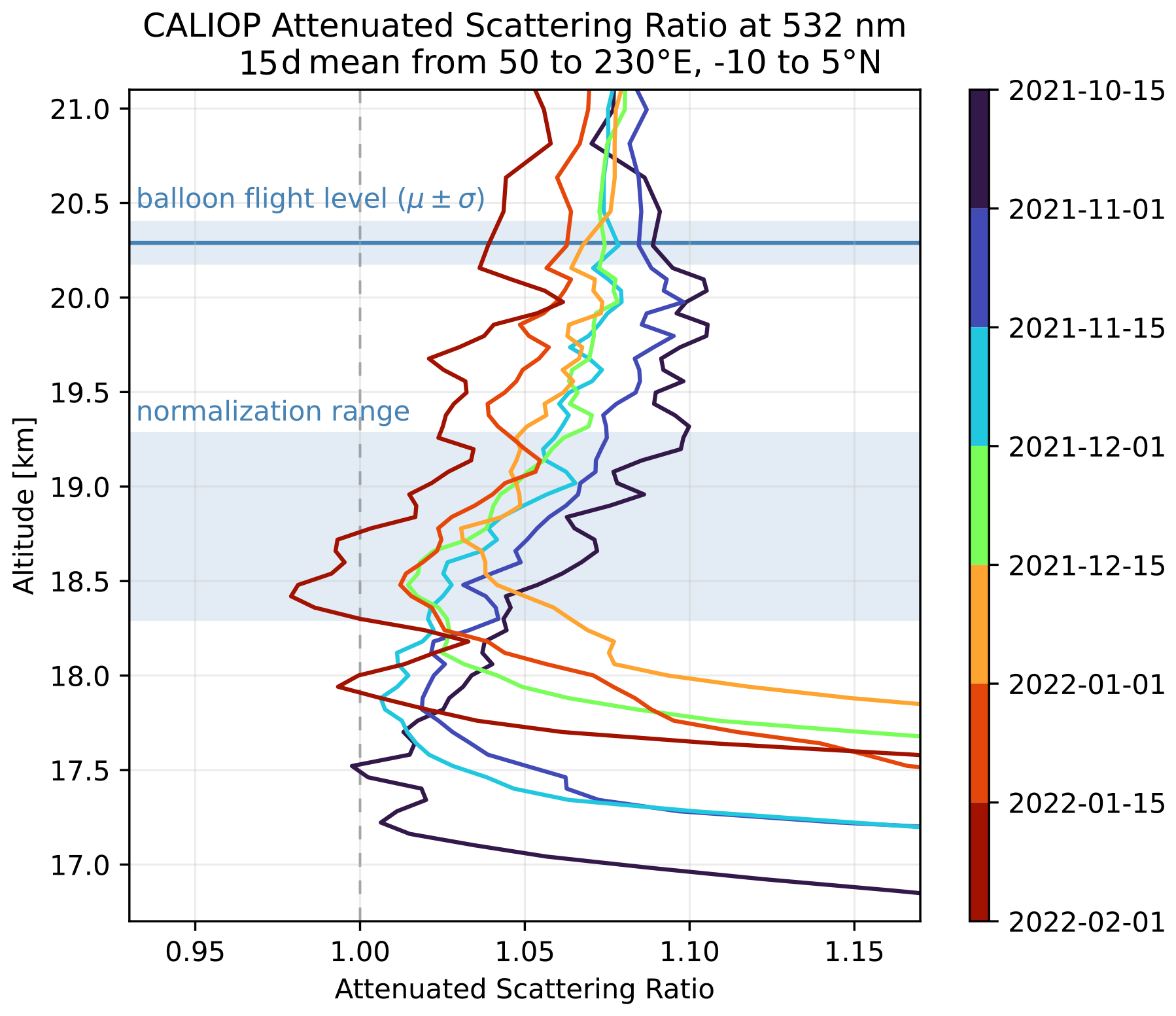
Figure 4 Mean CALIOP attenuated scattering ratio profiles averaged (50 to 230° E, −10 to 5° N) between October 2021 and January 2022. Each color line correspond to a mean over 15 d (red-blue color bar). The mean flight level of the balloon, and its variability is shown (horizontal blue line and upper blue-shaded area). The region where the normalization coefficient is computed (normalization range) is also shown (lower blue-shaded area).

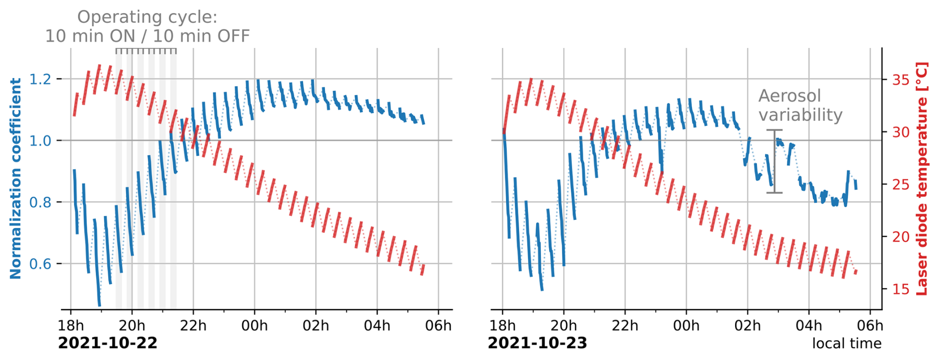
Figure 5 Time series of laser diode temperature (Celsius degrees, red line) and normalization coefficient (arbitrary unit, blue line) for two nights (local time) of flight ST2_C1_02_STR1. The normalization coefficient is the instrumental constant arbitrarily scaled to 1 at a given time. On the left panel (22 October 2021) the operating cycle (10 min ON/10 min OFF) is highlighted in grey.

Given the flight level of the balloons, it turns out that there is always a tenuous stratospheric aerosol layer between the gondola and the highests clouds observed by the lidar BeCOOL (Kremser et al., 2016). The variability of this layer has been investigated during the first Stratéole2 scientific campaign, using CALIOP nighttime overpasses, averaged between 50 to 230° E and −10 to 5° N, which are the closest to the flight tracks. Figure 4 illustrates the variability of the attenuated scattering ratio several kilometers below the flight level. The closest the ratio to 1, the better the approximation that Rayleigh scattering is prevailing. This is the case from 1 to 2 km below the flight level, the region we chose to estimate the value of K and compute B(r).

We calculated the value of K for each profile to account for the variations of power emitted by the laser diode and other overall transmission of the optical system. The left panel of Fig. 5 shows that K is driven by the laser diode temperature. During the night, given the limited insulation of the system, the stratosphere is cooling the system, whereas operating the laser diode during a cycle is warming it. The higher the laser diode temperature, the lower the value of K. The right panel of this Fig. 5 also shows this strong correlation, except between 2 and 4 h (local time). This is due to the presence of stratospheric aerosols.

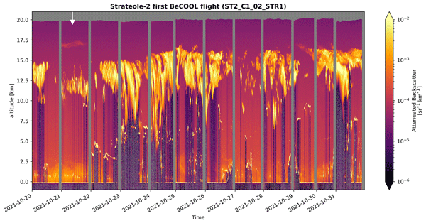
Figure 6 shows a cross section along the flight track of a stratospheric balloon of the attenuated backscatter B(r) for twelve consecutive nights. The atmosphere is cloud free above an altitude of 17.5 km. Several cloudy structures are observed below. The lidar is able to resolve them when they are optically thin enough. In these cases, BeCOOL is also observing the marine boundary layer and the ocean surface. When the laser beam encounters an optically thick structure, such as a large convective cloud, the signal is fully attenuated at some point within this cloud and the ocean surface is not observable. The white arrow on this figure is pointing towards the profile B(z)=β(z)[T(z)]² we are going to use to illustrate the inversion procedure to compute β(z) and the ability of BeCOOL to measure the optical depth τ of thin cirrus (left panel of Fig. 7). From now on, we will use the altitude z instead of the range r as the vertical coordinate.

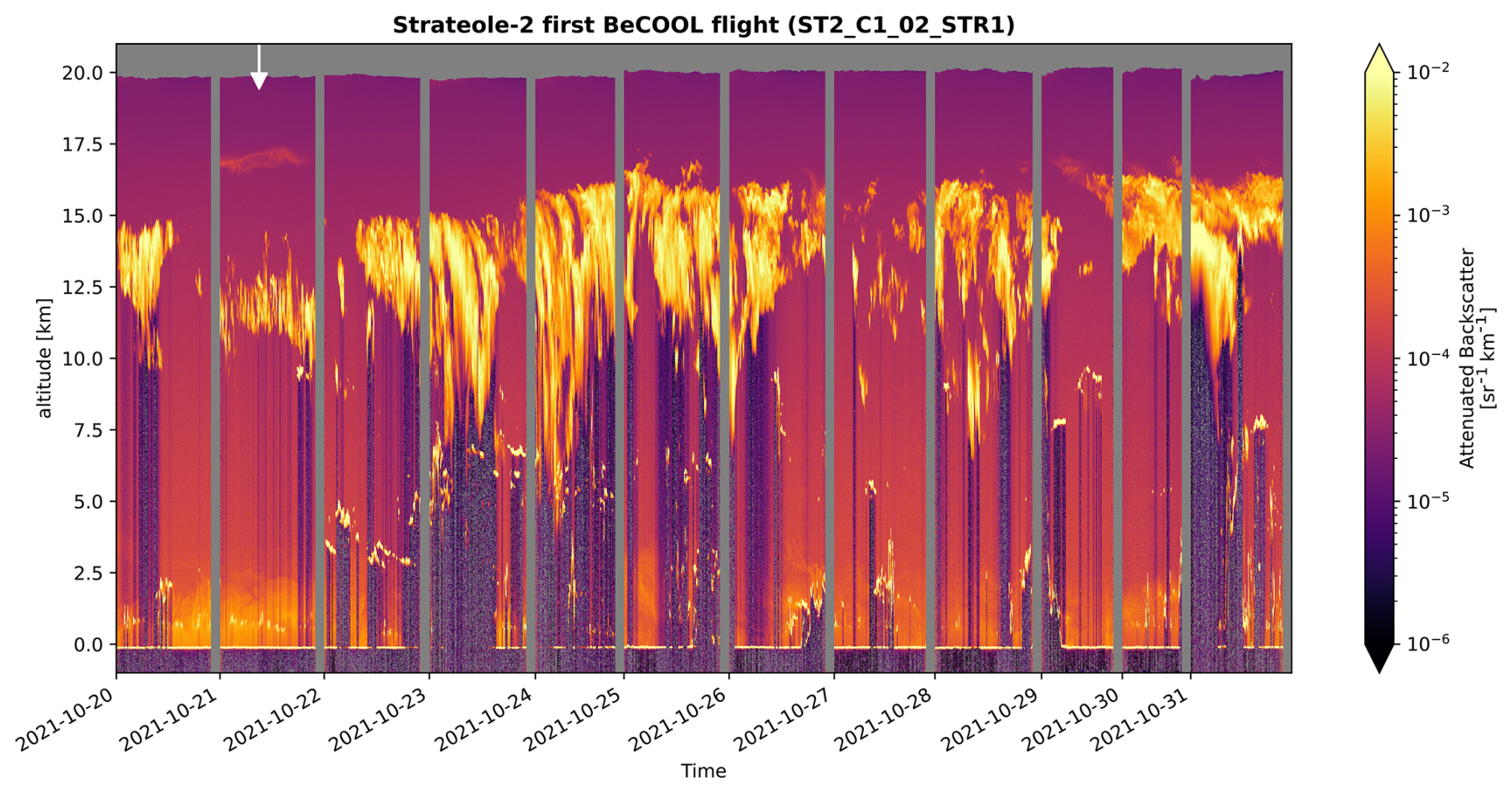
Figure 6 Lidar cross section (time vs. altitude) of the attenuated backscatter signal for the first BeCOOL flight of Stratéole2 2021–2022 scientific campaign, between 20 and 31 October 2021. Vertical grey lines separate two consecutive nights (BeCOOL is not operated during daytime). The upper horizontal grey-shaded area stands for no data. The upper white arrow is pointing the time corresponding to the profile retrieved in Sect. 4.

4 Backscatter profile and optical depth

The processing described in this section is performed on atmospheric profiles averaged over 10 min to improve the SNR. We use ERA5 meteorological profiles to compute the backscatter profile β_m(z), optical depth τ_m, transmission T_m and the attenuated backscatter profile $B_{\mathrm{m}}\left(z\right)={\mathit{\beta }}_{\mathrm{m}}\left(z\right)T_{\mathrm{m}}^{\mathrm{2}}\left(z\right)$ due to molecular (Rayleigh) scattering. We apply the Klett-Fernald procedure (Fernald et al., 1972; Fernald, 1984; Klett, 1981, 1985; Sasano et al., 1985) to derive the backscatter profile β(z) from B(z) , hence ${\mathit{\beta }}_{\mathrm{p}}\left(z\right)=\mathit{\beta }\left(z\right)-{\mathit{\beta }}_{\mathrm{m}}\left(z\right)$ and the optical thickness $\mathit{\tau }={\int }_{z_{\mathrm{b}}}^{z_{\mathrm{t}}}{\mathit{\alpha }}_{\mathrm{p}}\mathrm{d}z$ of clouds.

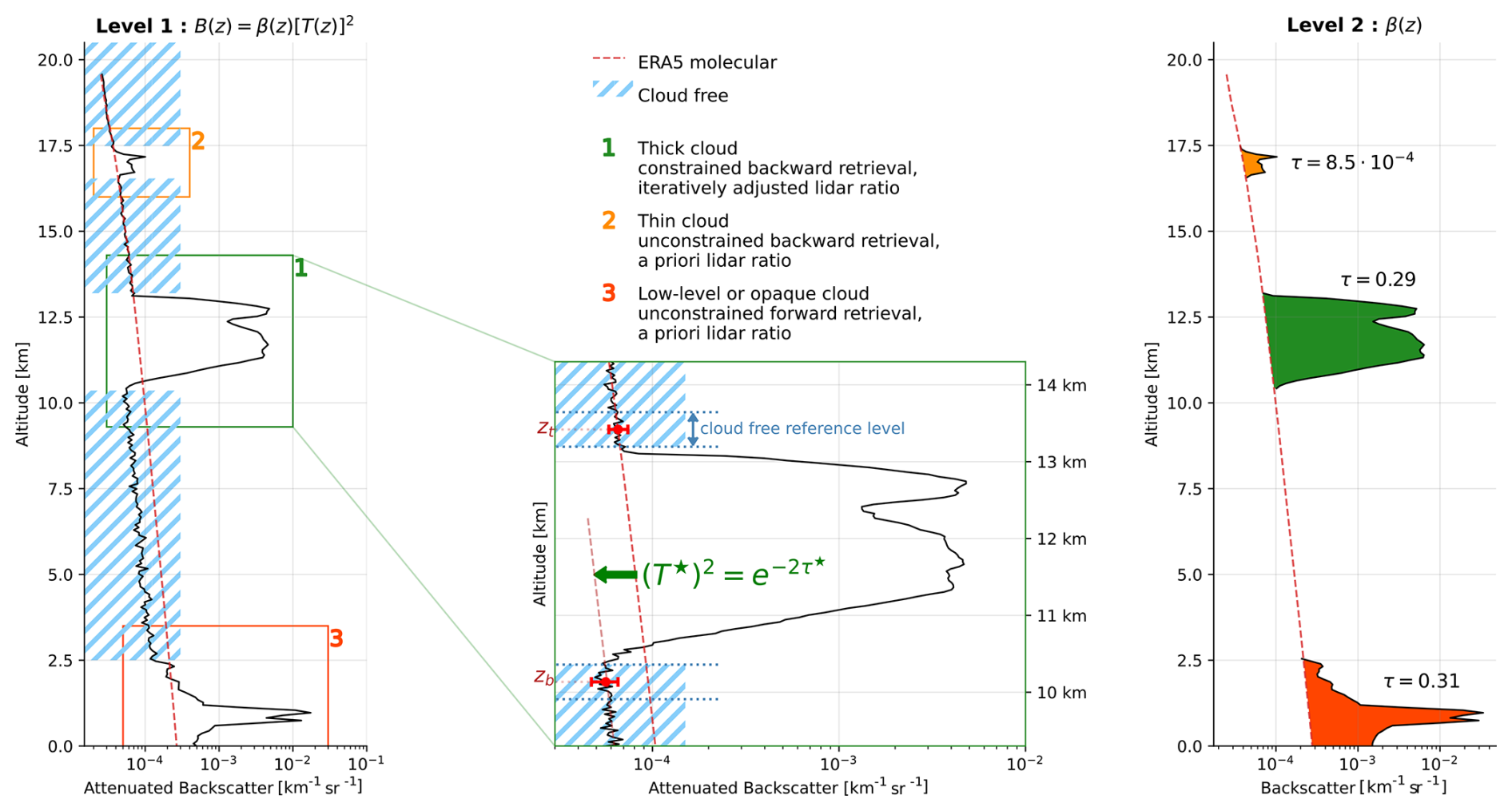
Figure 7 10-min averaged lidar profile on 21 October 2021 (white arrow on Fig. 6). The attenuated backscatter profile β[T(z)]² is plotted on the left panel, the backscatter profile β(z) on the right panel (the red dashed line is corresponding to β_m(z)). The middle panel is a zoom of the left panel for the cloud in the middle of the profile. The upper and lower red dots correspond respectively to the values of the averaged quantity (B^r) at the bottom (z_b) and the top (z_t) of the cloud. The red brackets show the lower (B^r−) and upper (B^r+) values of these reference quantities. The colored areas on the right panel materialize the optical depth for backward constrained retrieval (green), backward unconstrained retrieval (orange) and forward unconstrained retrieval (dark orange).

A preliminary step is the detection of clouds in each profile. We use the attenuated scattering ratio $B\left(z\right)/B_{\mathrm{m}}\left(z\right)$ to determine the cloud free regions of the atmosphere. When this ratio is significantly larger than one, a cloud is detected and we compute the altitude of its bottom (z_b) and of its top (z_t). The middle panel of Fig. 7 illustrates this procedure.

At these altitudes z_b and z_t, we average the attenuated backscatter signals $B^{\mathrm{r}}=\stackrel{\mathrm{‾}}{B\left(z\right)}$ using 10 consecutive points in the cloud free regions. These values will be used as reference values when applying the inversion procedure. In the same time, we compute upper (B^r+) and lower (B^r−) values of these quantities by adding or removing its standard error to the averaged reference value B^r. These reference values will be used when estimating the uncertainty of cloud optical depth (Sect. 5). They are plotted in red at the altitude z_b and z_t on the middle panel of Fig. 7.

To derive β(z) from B(z), i.e. to solve Eq. (1), we need to estimate a value of the lidar ratio $S={\mathit{\alpha }}_{\mathrm{p}}\left(z\right)/{\mathit{\beta }}_{\mathrm{p}}\left(z\right)$ and of η in cloudy layers. Two cases are to be considered for the choice of S when molecular scattering is observed above and below the cloud. When the attenuation of the signal by the cloud can be quantitatively estimated, it is possible to constrain the choice of S with an iterative procedure (Sect. 4.1, case 1 of Fig. 7). This is not the case when the cloud is optically thin (Sect. 4.2, case 2 of Fig. 7).

In cloudy layers, multiple scattering enhances the lidar signal collected by the reception channel (Platt, 1973; Nicolas et al., 1997; Garnier et al., 2015; Shcherbakov et al., 2024). The apparent cloud optical depth τ^* that is computed assuming no multiple scattering is smaller than the true one τ. A simple way to correct this underestimate is to consider a multiple scattering coefficient η (Platt, 1973) such as $\mathit{\tau }={\mathit{\tau }}^{*}/\mathit{\eta }$. As $\mathit{\tau }=\int S{\mathit{\beta }}_{\mathrm{p}}\mathrm{d}z$, the same correction applies to the lidar ratio S, which defines the apparent lidar ratio $S^{*}=\mathit{\eta }S$.

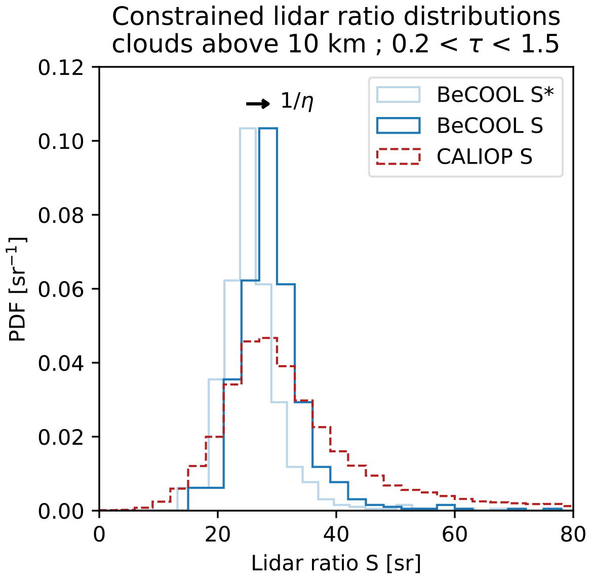
Figure 8 Probability distribution function (PDF) of the lidar ratio S. The light blue line corresponds to the PDF computed when the inversion of BeCOOL profiles is constrained, assuming no multiple scattering (the lidar ratio is noted S^* in this case). The red line corresponds to the PDF derived for the same category of clouds observed by CALIOP in the same region (optical depth between 0.2 and 1.5, altitude above 10 km). The dark blue line corresponds to the PDF computed when the inversion of BeCOOL profiles is constrained, assuming multiple scattering (η correcting factor).

4.1 Constrained retrieval

We first assume that there is no multiple scattering (η=1). We choose an a priori value of S^*. The integration of the lidar Eq. (1) is done backward, which is numerically more stable (Klett, 1981). A first profile of β(z) is computed, making it possible to estimate the apparent transmission of the cloud $T^{*}=e^{-{\mathit{\tau }}^{*}}$. This integration is done several time, the apparent lidar ratio S^* being iteratively adjusted until the value of T^* matches the observed one (see the middle panel of Fig. 7). In other words, starting with the initial condition B(z_b)=B^r(z_b), the apparent lidar ratio is adjusted until B(z_t)=B^r(z_t).

In a second step, we estimate the multiple scattering correction factor η, comparing BeCOOL's distribution of apparent lidar ratios S^* to CALIOP's distribution of lidar ratio S for clouds above 10 km, with an optical depth in the 0.2 to 1.5 range, over the tropical area explored by the BeCOOL flights (10° S to 5° N) between October 2021 and January 2022. Extensive work has been done to parameterize CALIOP's multiple scattering correction factor η using combined lidar and infrared radiometer observations (Garnier et al., 2012, 2015). We thus considered the values reported in CALIOP dataset (Level 2, V4-21, NASA/LARC/SD/ASDC, 2018), already corrected for multiple scattering, as the best estimate of the lidar ratio distribution.

Setting η=0.88 is reconciling the mode of these two distributions (see Fig. 8). It is also optimizing the overlap between the two distributions. This value is close to the one (0.80 ± 0.05) derived from dense low level water cloud observations by Mariage et al. (2017) with a similar instrument. Several adjustments of the value of η have been tested. We estimate that its uncertainty is about 0.1. The value of 0.88 has been used for η to compute the cloud optical depth τ and the backscatter profile (right panel of Fig. 7).

The distribution of the cloud optical depth computed with this method is shown on Fig. 9 (green line). Constrained retrieval can be used for an optical depth between 0.02 and 2. For larger values, BeCOOL is not powerful enough to go through the cloud. For smaller value, it is not possible to constrain the retrieval.

4.2 Unconstrained retrieval

When a cloud is optically thin, it is not possible to use the cloud free regions above and below this cloud to constrain its optical depth. The backward retrieval is only done once with an a priori lidar ratio (case 2 of Fig. 7). This value is derived from CALIOP’s successfully constrained lidar ratios over the time period and region covered by BeCOOL observations. These lidar ratios were vertically binned at 1 km resolution, and the most frequent value (mode) was retained for each altitude bin, producing a vertical profile of the most likely lidar ratios. The a priori lidar ratio used for BeCOOL's unconstrained retrieval is interpolated from this profile, and no further correction of the multiple scattering is needed.

The distribution of the cloud optical depth computed this way is shown on Fig. 9 (red line). Unconstrained retrieval is used for an optical depth between $\mathrm{2}\times {\mathrm{10}}^{-\mathrm{5}}$ and 0.2. The highest values (τ≳0.1) correspond to a limited number of cases of mid-level clouds for which the uncertainty of B^r is too large to estimate the apparent transmission. Comparing the constrained and unconstrained distribution, we consider an optical depth of $\mathrm{3}\times {\mathrm{10}}^{-\mathrm{2}}$ as the usual threshold value to switch from one method to the other.

When a cloud, such as a convective cloud, is optically so thick that the laser beam does not go through it or when we want to investigate cloud or aerosol layers close to the surface, it is also not possible to constrain the retrieval. Moreover, as there is no reference available below the cloud, we cannot use backward integration anymore. Switching to forward unconstrained retrieval, it is only possible to estimate a lower bound of the cloud optical depth (case 3 on Fig. 7). We will not develop this point here, as BeCOOL was first and foremost developed to investigate cirrus in the upper troposphere.

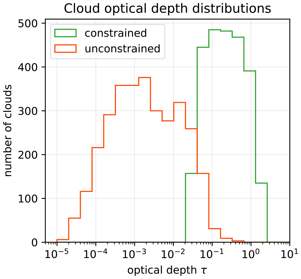
Figure 9 Distributions of retrieved cloud optical depth for the constrained (green line) and unconstrained (red line) backward retrievals.

5 Optical depth relative uncertainty

We now investigate the uncertainty attached to the former evaluation of the cloud optical depth $\mathit{\tau }={\int }_{z_{\mathrm{b}}}^{z_{\mathrm{t}}}{\mathit{\alpha }}_{\mathrm{p}}\mathrm{d}z$. We only consider the uncertainty due to the SNR variability in the cloud-free regions above and below a cloud. This is actually the uncertainty attached to the evaluation of the colored areas on the right panel of Fig. 7. For constrained retrieval, we assume that the multiple scattering coefficient and the lidar ratio are correctly evaluated. For unconstrained retrieval multiple scattering is negligible for optically thins clouds, but the uncertainty on the lidar ratio could be quite large (up to 40 % for ice clouds, Yorks et al., 2011).

Following Eq. (9) of Platt (1973), which implies to normalize the transmission T(z) at the top of the cloud (see Eq. 2), the uncertainty of the cloud optical depth related to the evaluation of the former areas can be estimated from the relationship between the integrated attenuated backscatter signal γ^′ and τ:

$$\begin{array}{}\text{(2)}& {\mathit{\gamma }}^{\prime }=\underset{z_{\mathrm{b}}}{\overset{z_{\mathrm{t}}}{\int }}\mathit{\beta }\left(z\right){\left[{\displaystyle \frac{T\left(z\right)}{T\left(z_{\mathrm{t}}\right)}}\right]}^{\mathrm{2}}\mathrm{d}z=\underset{z_{\mathrm{b}}}{\overset{z_{\mathrm{t}}}{\int }}\mathit{\beta }\left(z\right){\left[\widehat{T}\left(z\right)\right]}^{\mathrm{2}}\mathrm{d}z={\displaystyle \frac{\mathrm{1}-e^{-\mathrm{2}\mathit{\eta }\mathit{\tau }}}{\mathrm{2}\mathit{\eta }S}}\end{array}$$

Similarly to what is done for CALIOP (Liu et al., 2005, Fig. 7.1), we apply a trapezoid correction to estimate a particular-only contribution $\widehat{\mathit{\gamma }}$ to the total integrated attenuated backscatter γ^′ :

$$\begin{array}{}\text{(3)}& \begin{array}{rl}\widehat{\mathit{\gamma }}& =\underset{z_{\mathrm{b}}}{\overset{z_{\mathrm{t}}}{\int }}{\mathit{\beta }}_{\mathrm{p}}\left(z\right){\left[\widehat{T}\left(z\right)\right]}^{\mathrm{2}}\mathrm{d}z={\mathit{\gamma }}^{\prime }\\ & -{\displaystyle \frac{\mathrm{1}}{\mathrm{2}}}{\displaystyle \frac{B^r\left(z_{\mathrm{b}}\right)+B^r\left(z_{\mathrm{t}}\right)}{{\left[T\left(z_{\mathrm{t}}\right)\right]}^{\mathrm{2}}}}(z_{\mathrm{t}}-z_{\mathrm{b}})\end{array}\end{array}$$

Using upper and lower bound of the attenuated backscatter reference values at the bottom and of the top of the cloud (Sect. 4) and going back to Eq. (3), we can evaluate for each cloud the upper and the lower bound of $\widehat{\mathit{\gamma }}$, hence its relative uncertainty $\frac{\mathit{\delta }\widehat{\mathit{\gamma }}}{\widehat{\mathit{\gamma }}}=\frac{{\widehat{\mathit{\gamma }}}^{+}-{\widehat{\mathit{\gamma }}}^{-}}{\widehat{\mathit{\gamma }}}$, with ${\widehat{\mathit{\gamma }}}^{+}={\mathit{\gamma }}^{\prime }-\frac{\mathrm{1}}{\mathrm{2}}\frac{B^{\mathrm{r}-}\left(z_{\mathrm{b}}\right)+B^{\mathrm{r}-}\left(z_{\mathrm{t}}\right)}{{\left[T\left(z_{\mathrm{t}}\right)\right]}^{\mathrm{2}}}(z_{\mathrm{t}}-z_{\mathrm{b}})$ and ${\widehat{\mathit{\gamma }}}^{-}={\mathit{\gamma }}^{\prime }-\frac{\mathrm{1}}{\mathrm{2}}\frac{B^{\mathrm{r}+}\left(z_{\mathrm{b}}\right)+B^{\mathrm{r}+}\left(z_{\mathrm{t}}\right)}{{\left[T\left(z_{\mathrm{t}}\right)\right]}^{\mathrm{2}}}(z_{\mathrm{t}}-z_{\mathrm{b}})$. Proceeding this way, the uncertainty on the cloud optical depth is due to the uncertainty of the contribution of Rayleigh scattering to γ^′.

When the optical depth is large enough, the retrieval is constrained retrieval, and we have ${\mathit{\gamma }}^{\prime }\simeq \widehat{\mathit{\gamma }}$. Defining the auxiliary variable $y=\mathrm{1}-\mathrm{2}\mathit{\eta }S\widehat{\mathit{\gamma }}$, we get $\mathit{\tau }=-\frac{\mathrm{1}}{\mathrm{2}\mathit{\eta }}\ln \left(y\right)$, and $\frac{\mathit{\delta }\mathit{\tau }}{\mathit{\tau }}=\frac{\mathit{\delta }y}{y\ln y}$. For these clouds the distribution of the relative uncertainty against cloud optical depth is plotted in green on the Fig. 10. The colored areas ranging from light to dark green correspond to 90 % of the observations during the Stratéole2 campaign. The darker the shade, the denser the distribution of the observations in the region, the darkest area containing for instance 10 % of the observations. In agreement with Fig. 9 we find that the cloud optical depth distribution for constrained retrieval peaks near 0.2, with a relative uncertainty smaller than 1 %. Considering 90 % of the points, we see that for clouds with an optical depth ranging from 2 to $\mathrm{3}\times {\mathrm{10}}^{-\mathrm{2}}$ the relative uncertainty $\mathit{\delta }\mathit{\tau }/\mathit{\tau }$ is smaller than 5 %.

For optically thin clouds whose optical depth is smaller than $\mathrm{3}\times {\mathrm{10}}^{-\mathrm{2}}$ the retrieval is unconstrained, multiple scattering is negligible and the cloud transmission T is close to 1. As a result: $\mathit{\tau }\simeq S\widehat{\mathit{\gamma }}$ and $\frac{\mathit{\delta }\mathit{\tau }}{\mathit{\tau }}=\frac{\mathit{\delta }\widehat{\mathit{\gamma }}}{\widehat{\mathit{\gamma }}}$. For these clouds, the distribution of the relative uncertainty against cloud optical depth is plotted in red on the Fig. 10. For these clouds, the smaller the optical depth, the larger its relative uncertainty. Where observations are the denser (dark red area), the relative uncertainty is about 1 % for an optical depth of 0.01, and about 30 % for an optical depth of 10⁻⁴. Considering 90 % of the observations (red colored areas), we see that the relative uncertainty only due to the SNR variability can be as large as 90 %.

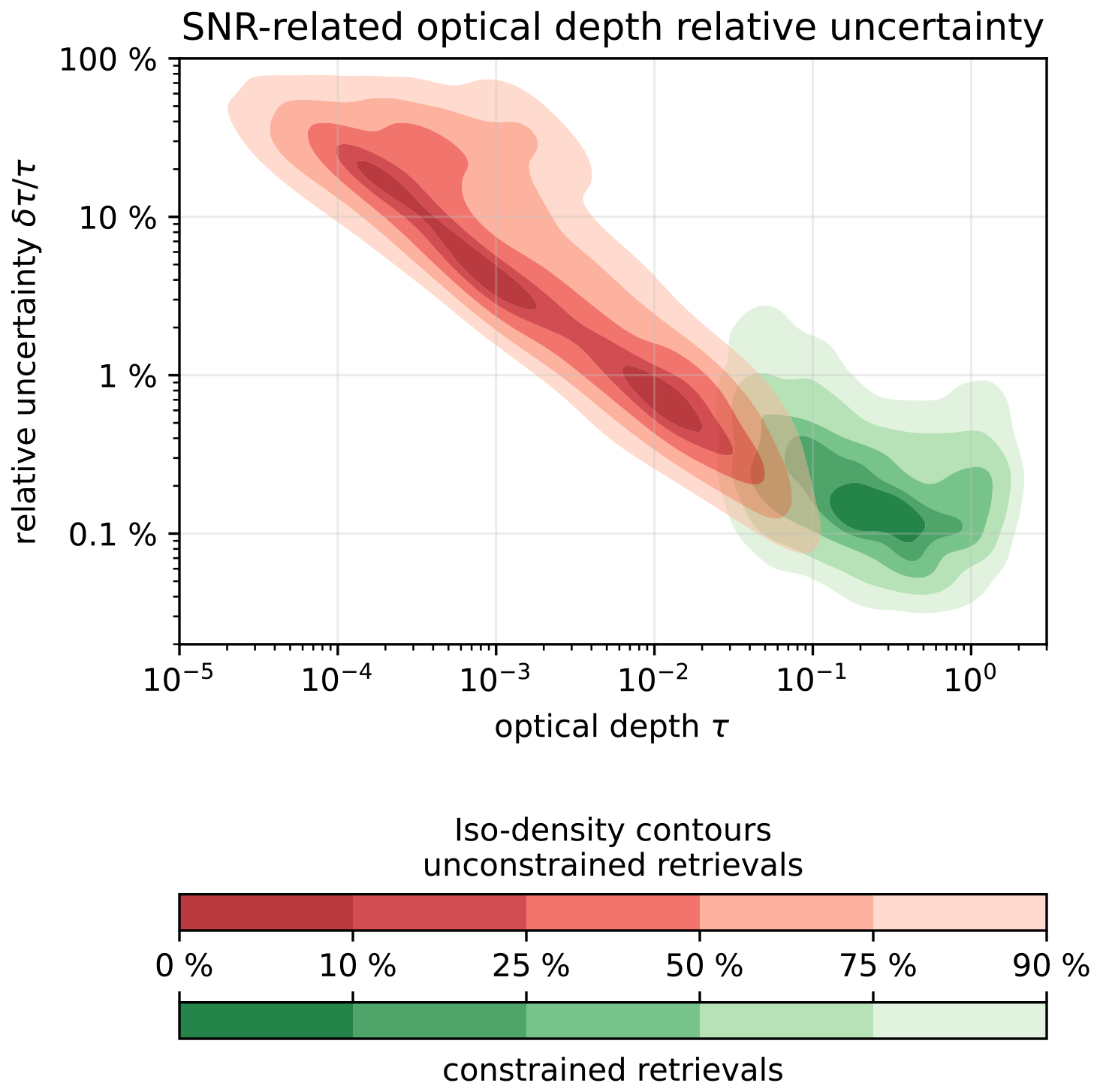
Figure 10 SNR-related cloud optical depth relative uncertainty against cloud optical depth for constrained (green contours) and unconstrained (red contours) backward retrievals. The darker the contour, the larger the number of measurements. For each color, the total colored area correspond to 90 % of the observations. For each color, the darkest contour corresponds to 10 % of the observations, where measurements are the denser.

6 Conclusions and perspectives

BeCOOL has been designed to be operated onboard a small gondola in the stratosphere. It can work autonomously for several months. It weights less than 6 kg. It requires on average a power supply of 8 W if the microlidar is operated continuously, and of 4 W with a 50 % duty cycle.

This backscatter microlidar operating at 802 nm has been successfully deployed during the 2021–2022 Stratéole2 field campaign, first and foremost to monitor cirrus clouds. Given the slow motion of stratospheric balloon, SNR is high enough to sample thin clouds with an optical depth ranging from $\mathrm{2}\times {\mathrm{10}}^{-\mathrm{5}}$ to 2 at 802 nm. When the cloud optical depth is larger than $\mathrm{3}\times {\mathrm{10}}^{-\mathrm{2}}$, its relative uncertainty is smaller than 5 %. For very thin clouds this uncertainty can be as high as 90 %. Moreover on should also consider the uncertainty attached to choice of the lidar ratio when the retrieval of the lidar data is not constrained.

Thanks to this very high sensitivity to low optical depths, BeCOOL revealed a significant population of thin cirrus in the Tropical Tropopause Layer (TTL) that were not detected by the spaceborne lidar CALIOP. Such ultrathin cirrus (optical depths below $\mathrm{2}\times {\mathrm{10}}^{-\mathrm{3}}$) are observed in 23 % of the lidar profiles (Lesigne et al., 2024). Balloon-borne lidar observations therefore offers a unique observational window on clouds that have remained largely undetected so far. Furthermore, the large scale impact of cirrus clouds, whether through radiative heating or water redistribution within the TTL, depends on their lifetime, which cannot be investigated from spaceborne measurements that mainly provide quasi-instantaneous snapshots of clouds over large spatial scales. The slow drift of the balloons over the clouds enables the investigation of their lifetime. The estimated mean lifetime of TTL cirrus clouds is about 6 h, and 70 % of the cloud cover is associated with clouds persisting longer than 12 h (Lesigne et al., 2025). Finally, the high vertical resolution of BeCOOL measurements highlights the fine-scale morphology of TTL cirrus, bringing new insights into the interactions between cirrus microphysics and small-scale dynamics, which are currently investigated using Lagrangian microphysics simulations.

Four BeCOOL instruments will be deployed during the next Stratéole2 field campaign (winter 2026–2027). Comparing the datasets of the two campaigns, it will be possible to discuss the variability of the cloud distribution. If the balloons are circumnavigating the globe, it will also be possible to investigate the topography of convective clouds over the continents, using the lidar as a telemeter.

New instrumental developments are also under way, either to improve the performances of the microlidar or to operate it in synergy with other instruments. The combination of BeCOOL with a radar will make it possible to investigate deep convection and mixed-phased clouds. Its deployment with a radiometer will be very useful to study the radiative impact of upper level clouds. Regarding the microlidar itself, the priority in terms of new developments is given to its operation during daytime and at higher altitudes in the stratosphere to study the stratospheric aerosol layer and monitor natural or anthropogenic perturbation of this region.