the Creative Commons Attribution 4.0 License.
the Creative Commons Attribution 4.0 License.
 | 06 Jul 2018
Remote sensing of aerosols with small satellites in formation flight
Kirk Knobelspiesse
Sreeja Nag
Determination of aerosol optical properties with orbital passive remote sensing is a difficult task, as observations often have limited information. Multi-angle instruments, such as the Multi-angle Imaging SpectroRadiometer (MISR) and the POlarization and Directionality of the Earth's Reflectances (POLDER), seek to address this by making information-rich multi-angle observations that can be used to better retrieve aerosol optical properties. The paradigm for such instruments is that each angle view is made from one platform, with, for example, a gimballed sensor or multiple fixed view angle sensors. This restricts the observing geometry to a plane within the scene bidirectional reflectance distribution function (BRDF) observed at the top of the atmosphere (TOA). New technological developments, however, support sensors on small satellites flying in formation, which could be a beneficial alternative. Such sensors may have only one viewing direction each, but the agility of small satellites allows one to control this direction and change it over time. When such agile satellites are flown in formation and their sensors pointed to the same location at approximately the same time, they could sample a distributed set of geometries within the scene BRDF. In other words, observations from multiple satellites can take a variety of view zenith and azimuth angles and are not restricted to one azimuth plane as is the case with a single multi-angle instrument. It is not known, however, whether this is as potentially capable as a multi-angle platform for the purposes of aerosol remote sensing. Using a systems engineering tool coupled with an information content analysis technique, we investigate the feasibility of such an approach for the remote sensing of aerosols. These tools test the mean results of all geometries encountered in an orbit. We find that small satellites in formation are equally capable as multi-angle platforms for aerosol remote sensing, as long as their calibration accuracies and measurement uncertainties are equivalent. As long as the viewing geometries are dispersed throughout the BRDF, it appears the quantity of view angles determines the information content of the observations, not the specific observation geometry. Given the smoothly varying nature of BRDF's observed at the TOA, this is reasonable and supports the viability of aerosol remote sensing with small satellites flying in formation. The incremental improvement in information content that we found with number of view angles also supports the concept of a resilient mission comprised of multiple satellites that are continuously replaced as they age or fail.
- Article
(9314 KB) - Full-text XML
- BibTeX
- EndNote


Atmospheric aerosols play a potentially significant role in the global climate, both through direct scattering and absorption of solar radiation and indirectly by modifying clouds and local meteorology. Additionally, aerosols contribute the largest overall net radiative forcing uncertainty (IPCC, 2013) due in part to insufficiently accurate and complete observations on a global scale (Mishchenko et al., 2004). This is because most aerosol remote sensing is underdetermined, meaning there is less information contained in the observations than necessary to accurately extract the necessary aerosol descriptive parameters. The aerosol remote sensing community is therefore developing instruments that maximize “information content” (IC), by observing a scene at multiple wavelengths, viewing angles and polarimetric states (Kokhanovsky et al., 2015).
Notable examples of instruments that make use of multi-angle observations include the Multi-angle Imaging SpectroRadiometer (MISR) and the POlarization and Directionality of the Earth's Reflectances (POLDER). MISR, launched on the NASA Terra spacecraft in 1999, observes in four spectral bands and nine view angles spread in the flight track direction (Diner et al., 1998; Kahn et al., 2005). As of 2016, MISR is still operational and has been collecting data for more than 16 years. Three versions of POLDER have collected data, the most recent and longest lived on the French CNES (Centre National d'Etudes Spatiales) PARASOL (Polarization and Anisotropy of Reflectance for Atmospheric Sciences coupled with Observations from a Lidar) spacecraft, launched in 2004 and removed from orbit in 2013. POLDER observed a scene with up to 16 views in the along-track direction, with nine spectral channels at visible and near-infrared wavelengths. Three of those channels were also sensitive to linear polarization (Dubovik et al., 2011; Fougnie et al., 2007; Hasekamp et al., 2011; Tanré et al., 2011). The Clouds and Earth Radiant Energy System (CERES) instruments have the capability to scan in an arbitrary solar-sensor azimuth plane, although such systems do not collect multiple angle views of the observed location at the same time (Smith et al., 2011; Wielicki et al., 1996).
The instruments described above are what we call “multi-angle” platform instruments, since all measurements are made from one instrument. New and rapidly developing technology has created the possibility that several individual instruments can make a multi-angle observation in an entirely different manner. We consider formations of single-view angle instruments in orbit, coordinated to observe the same point simultaneously. This approach may be advantageous for a variety of engineering, cost or operational reasons. A formation of small satellites can make multi-spectral measurements of a ground spot at multiple angles simultaneously as they pass overhead using instruments with narrow fields of view in controlled formation flight (Nag et al., 2016, 2017a). Figure 1 shows a graphic for a multiple satellite case, where the relative positions of the satellites do not need to be tightly controlled, but their relative attitudes do. Our proposed concept is aimed at improving only the angular coverage of measurements because the images collected by the satellites are expected to overlap. The spatial and temporal coverage of the formation will depend on the swath of any single sensor and can be improved by flying a constellation of such formations
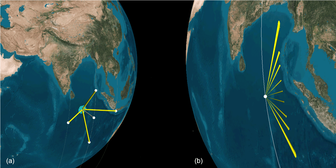
Figure 1Illustration of the observation geometry of five single-view-angle satellites flying in formation (a) and a nine-view multi-angle single satellite (b). The satellites in formation flight simultaneously observe the same ground spot at five different zenith and azimuth angles. The relative positions of these satellites do not need to be tightly controlled, but their relative attitudes do. The multi-angle satellite observes in the along-track direction, so that a ground spot is observed from nine angles as the satellite passes overhead. These observations occur within the same azimuth plane at various zenith angles.
Aerosol optical properties are determined from an orbital measurement, y, that is a vector containing reflectances for various wavelengths, polarization states and geometries. Such a vector represents a sample of the top of atmosphere (TOA) bidirectional reflectance distribution function (BRDF). As defined in Nicodemus et al. (1977), the BRDF is the geometrically and spectrally resolved ratio of scattered to incident light:
where L is the radiance in units of W m−2 sr−1 and E is the irradiance in units of W m−2. The BRDF is a function of solar zenith angle θs, view zenith angle θv, solar azimuth angle ϕs, view azimuth angle ϕv, and wavelength λ. Note that L and E could contain vectors describing polarization state, in which case the above equation would represent the bidirectional polarization distribution function (BPDF) (Nadal and Breon, 1999). For the earth, BRDF is typically symmetric about the solar azimuth angle, so that ϕs and ϕv can be condensed to (Knobelspiesse et al., 2008), which was what was used here. The algorithm used to determine the optimal formation flight architectures, which assessed their ability to determine BRDF (Nag et al., 2015) or any BRDF dependent product (Nag et al., 2016), did take the asymmetric azimuth nature into account. In practice, observations are often expressed as a unitless quantity (reflectance; see Sect. 3.3) that has been integrated over solar geometries and represents a finite view solid angle.
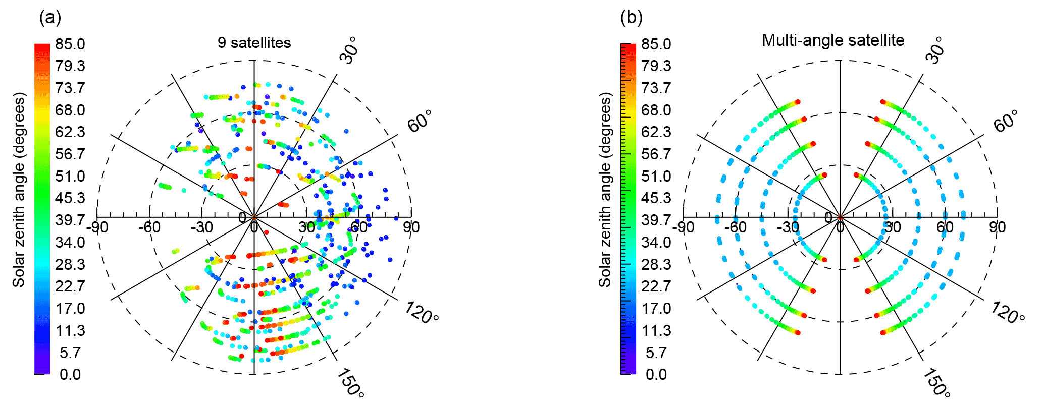
Figure 2Simulated viewing geometries in 1 day for nine single-view satellites in formation flight (a) and a multi-angle satellite with nine views in the along-track direction (b). View zenith angle (θv) is indicated in the radial coordinate dimension, while the relative solar – view angle azimuth () is in the angular dimension. Solar zenith angle (θs) is expressed by color. We limited θsto< 85∘; 106 and 119 scenes for the nine-satellite and multi-angle satellite configurations met this criteria in our tests, respectively.
The TOA BRDF or BPDF depend upon interactions between incoming solar radiation and the gases, aerosols, clouds and surfaces that comprise an earth scene. They therefore can contain information about the optical properties and quantities of these constituents. A generalized way to retrieve these values is to compare the measurements, y, to the computed result of a radiative transfer (RT) model simulation. Such models compute a BRDF, which is sampled to simulate measurement vector y′ given a set of descriptive geophysical scene parameters, x, and other ancillary information b. y and y′ are then compared, and x iteratively adjusted (by a variety of methods) until the closest match can be found. The ability to successfully converge to a solution depends on measurement system characteristics, RT model fidelity and other factors. In this study, we are concerned with the impact that measurement characteristics, specifically observation geometry, have on the ability to accurately determine x. These parameters are indicated in bold in Table 2, whereas other parameters held fixed in the analysis can be considered components of b. The limited IC of the system drives the partition between x and b in our analysis and is why we choose to compare IC relative to a single multi-angle instrument baseline. The b applied in all cases is the same. In practice, real retrievals may require the use of aerosol models, which address limited IC by constraining parameter space.
Figure 2 illustrates the BRDF sampling differences between a formation of instruments and a multi-angle instrument. Results were generated by simulations of orbit characteristics described in Sect. 2.1, with roughly 100 observations each for a formation of nine satellites (left) and a multi-angle instrument with a geometry similar to that of the MISR instrument (right). The multi-angle satellite observes the BRDF or BPDF in a much more ordered manner than the formation of nine satellites: observations are made at a fixed θv, and solar zenith angles covary with ϕ. Observations are not made in the solar principal plane (where ϕ=0∘) except at nadir (θv=0∘). The nine-satellite configuration, however, is far less uniform. Many observations are made in the solar principal plane (although often with high θs). The multi-angle instrument thus has a measurement vector, y, that is much more uniformly ordered than that of the formation of single-view instruments.
The goal of this paper it to examine these differences and determine whether there are advantages (or disadvantages) of using formations of multiple satellites with single but adjustable view compared to multi-angle instruments. Section 2.1 describes the systems engineering model used to select the satellite formation characteristics and observation geometries expressed in Fig. 2. Section 2.2 describes the IC assessment technique, which uses instrument characteristics and RT model simulations to predict the uncertainty in the retrieved x. Section 3 provides details on the characteristics of the systems engineering models, RT model and IC assessment. Section 4 contains the results of this assessment, while Sect. 5 concludes.
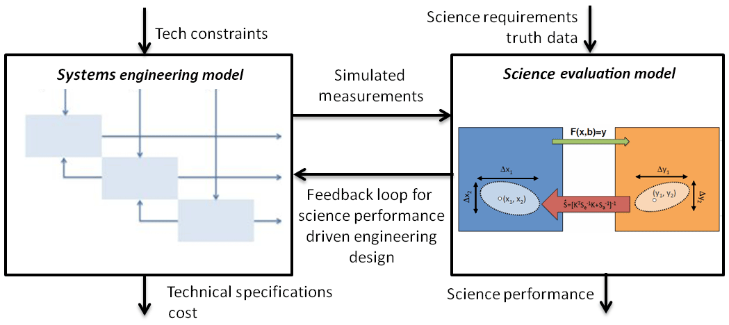
Figure 3The relationship between the systems engineering model and the science evaluation model from Nag et al. (2016). The engineering model takes in the mission's technical constraints and outputs optimized technical specifications, simulated measurements and cost for hundreds of simulated architectures. The science evaluation model performs information content analysis on the simulated measurements based on science requirements and reference data and outputs science performance and error values for each architecture.
An architecture is defined as a unique combination of design variables such as number of satellites, their orbit parameters, the spectrometer or polarimeter payload's field of view, pixel size, number of spectral bands, spectral resolution and communication bands for downlink. The methodology employed to assess the optimal architectures and validate their aerosol retrieval capabilities couples systems engineering and IC analysis, a method of science performance evaluation. A trade space of architectures can be analyzed by varying the design variables in the systems engineering model and assessing its effect on science products using IC assessment, as shown in Fig. 3. The left-hand box generates multiple architectures by permuting different values of the design variables, sizing them to check their technical feasibility and costing them relative to one another. The systems engineering model can be simulated over any time horizon and divided into appropriate time steps. The right-hand box evaluates the IC that can be retrieved from the angular spread of measurements, at every instant of time, for every architecture. We perform this assessment using Bayesian statistical techniques that connect simulated scenes to the potential geophysical parameter retrieval ability of a selected architecture. This assessment is performed for a variety of types of scenes, so that the aggregate result is more representative of global conditions.
2.1 Systems engineering model
In the last few years, several small satellite constellations with atmospheric science sensors have successfully flown (e.g., the Cyclone Global Navigation Satellite System or CYGNSS; Ruf et al., 2012) or have been funded for imminent flight (e.g., TROPICS; Blackwell, 2015). While such systems demonstrate capability to house science payloads, the satellites in these constellations do not need to coordinate their measurement operations, and their attitude is fixed in local space. Our proposed formation requires that all satellites point to the same target at approximately the same time, which demands agility and consistent attitude control. Simulation studies have demonstrated that it is possible to maintain the orbits and orientation of small satellites in such a formation, using commercially available propulsion and control systems (Nag et al., 2016).
As described in previous literature (Nag et al., 2017a), a modular systems engineering model is capable of simulating hundreds of small satellite formation flight architectures, constrained by current small spacecraft capabilities such as launch availability, propulsive correction capability and commercial attitude control as well as by BRDF measurement requirements such as medium spatial resolution and full hemispherical angular spread. Such a model automatically balances technical trades between conflicting variables such as required ground pixel size and control stability, required pixel size and off-pointing angles, or number of orbital planes and off-track angles. Therefore, the formation flight architectures generated by the model are optimized to ensure they are technically feasible. The outputs corresponding from each architecture are (among others), the angular spread of measurements on the ground at any given simulation instant, where the number of measurements will be equal to the number of satellites (Fig. 1). Figure 3 summarizes the coupling between the systems engineering model, which generates spacecraft formation architectures, and the science evaluation model, which assesses the IC within the angular and temporal measurements that the architectures are capable of making. The coupling may be an iterative one where science performance errors are used to inform better engineering design.
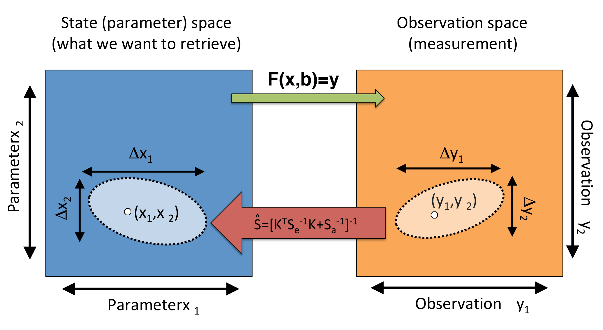
Figure 4This figure is an illustration of information content assessment concepts. We consider a state space (blue) representing all possible geophysical parameter values. Each point within this space is a plausible geophysical state, expressed as the vector x. There is a corresponding space representing measurements by an observing system (orange). The vector y in this space represents a measurement. Practically, all measurements have uncertainty, represented by the light orange portion of observation space. We are interested to learn what uncertainty volume (light blue) corresponds to the measurement uncertainty volume in state space. To find this, we use the forward model (, green arrow), which produces a simulated observation given a geophysical state. Since our forward model is highly nonlinear, it is not easily inverted to go in the other direction, from observation space to state space. However, the sensitivity of this forward model (the Jacobian, K), if assumed linear for small perturbations, can be combined with knowledge of the measurement uncertainty, Sϵ, and prior knowledge of the state space, Sa, to determine the retrieval error covariance matrix, . This is indicated by the red arrow and must be computed for several locations within the spaces because of the nonlinearity in the forward model to achieve a realistic understanding of these relationships. In practice, we work with systems with much higher dimensionality than two, which is used here for clarity.
This paper focuses on only those design variables in the systems engineering model that pertain to orbital design and payload pointing strategies of a satellite formation. Specifically, these variables are number of satellites, altitude and inclination of the chief orbit, the relative differences between the Keplerian elements of different satellites and strategies for payload pointing for obtaining multi-angular images simultaneously. Three potential strategies or imaging modes are
-
Fixed reference satellite, wherein one satellite always points nadir while others point at the ground spot below the reference satellite;
-
Variable reference satellite, which is the same as 1 except that the reference satellite varies;
-
Tracking mode, where all satellites track pre-defined ground points as they emerge from and disappear over the horizon.
The third imaging mode obviously provides the most angular coverage, at the cost of spatial coverage because only a small set of ground points can be tracked with one formation of satellites.
We have not optimized the design variables in this paper, but instead have used formation architecture designs that have been shown to be optimum for land surface (not TOA) BRDF estimation from space, as averaged over 1 day of simulation (Nag et al., 2015). The architectures were compared to each other on the basis of root-mean-squared (rms) BRDF errors, which were computed against airborne data collected over years of campaigns by the NASA Goddard Space Flight Center's Cloud Absorption Radiometer, or CAR (Gatebe and King, 2016). Since the CAR can fly around any ground spot in circles with adjustable altitude, it can collect hundreds of thousands of angular measurements and estimate BRDF more accurately than any other aerial or space instrument. CAR data can therefore be assumed as a standard to compare other measurement techniques for BRDF and its dependent products. The airborne data were organized by surface type, whose global distribution was obtained from the MODIS Global Land Cover Facility (Friedl et al., 2010). The errors were derived from the BRDF retrieved at every instant by the formation, depending on the surface type expected to be seen by the formation at that particular instant. Nag et al. (2016, 2017a) detail the measurement requirements for surface BRDF observations and the process of computing rms errors with respect to reference data (e.g., CAR) so as to optimize formation designs that minimize errors. Nag et al. (2017b) demonstrate that commercial payloads, flown at the proposed altitude and angular ranges, are capable of meeting the above measurement requirements.
2.2 Information content analysis
We use an IC assessment method that applies Bayesian statistical techniques to connect measurements to the expected retrieval success of geophysically relevant parameters. This technique is described for atmospheric remote sensing by Rodgers (2000) and more specifically for multi-angle polarimetric remote sensing of aerosols by, for example, Hasekamp and Landgraf (2007), Knobelspiesse et al. (2012) and Xu and Wang (2015). This analysis uses the same software for RT and other computations as Knobelspiesse et al. (2012).
Figure 4 is a conceptual illustration of the IC analysis technique. We consider two multidimensional spaces. The state (or parameter) space spans possible geophysical parameter values (left box in Fig. 4), while the observation space spans possible observed measurement values (right box). Geophysical reality may be expressed by a point within state space represented by the vector x, where each element contains parameters describing aerosol size distribution, refractive index, etc. (see Table 2 for a list of parameters used in this analysis). This corresponds to a point represented by the vector y in observation space, where each element contains the measured reflectance or radiance for a particular geometry and spectral channel. Connecting the two is the forward (RT) model, (), which produces a simulated observation, y, given geophysical parameters, x, and other required model inputs, b. The difference between x and b, for the purposes of remote sensing, is that the former are the parameters one wishes to retrieve, while the latter are required to simulate an observation (such as total atmospheric pressure), but are either parameterized or specified with ancillary data. As we shall see later, we have structured our IC analysis to minimize the impact of changes in b for different systems.
All measurements have uncertainty, so an observation is really an expression of a volume within observation space, represented by both y and uncertainties about those points . We are concerned with how that volume in observation space maps to a volume in parameter space, as it shows the utility of a measurement system. This relies on both instrument characteristics and the relationship between state and observation spaces, which we explore with our RT model. We express this by calculating the retrieval error covariance matrix, :
where is the uncertainty volume surrounding x. The diagonals of this square matrix correspond to squared uncertainties associated with each parameter in x, while off-diagonal elements are the covariances between them. The retrieval error covariance matrix depends on the observation error covariance matrix, Sϵ, the a priori error covariance matrix, Sa, and the Jacobian matrix, K (T denotes the transpose, and −1 the inverse). The observation error covariance matrix, Sϵ, corresponds to the area surrounding y in Fig. 4, where diagonals are the squared uncertainties of each measurement in y, and off-diagonal elements are their covariance. This matrix contains instrument calibration accuracies, typically the largest source of uncertainty for aerosol remote sensing instruments. The a priori error covariance matrix, Sa, represents knowledge of the parameters before a measurement. This is the boundary of possible state space, the total area (blue in Fig. 4) of that space. It is defined in a similar fashion as and Sϵ, where diagonals are the squared prior parameter uncertainty, and off-diagonals their covariance. The Jacobian matrix K is the forward model sensitivity, estimated with a forward difference:
which assumes F(x) is linear for the perturbation x′. This is reasonable for our RT model since we use small perturbations, although F(x) is highly nonlinear overall. To compute the Jacobian, we must execute the RT model for x, and then again with a perturbation for each element in x. Wang et al. (2014) show an example of an IC assessment system that uses a linearization of the forward model to compute the Jacobian, which will be more robust if F(x) is nonlinear over small perturbations. To assess the overall IC of a system we also must compute using an assemblage of different Jacobians, each partial derivative estimated at various locations within state space. In other words, we compute Eq. (2) for many different scenes (defined as a point in state space connected to a point in measurement space by the forward model), with different aerosol optical properties, and draw conclusions based on the aggregate result. To some extent, multiple assessments may also cancel inaccuracies due to the linearity assumption over small perturbations as well. Because we have no justification to do otherwise, the a priori error covariance matrix, Sa, is constant throughout the multiple assessments of .
can also be used to predict the uncertainty of parameters that are not explicitly retrieved, but derived from retrieved parameters (Hasekamp and Landgraf, 2007). If the definition of a parameter, a, is generalized such that a=G(x), then the uncertainty for a is
This presumes that G(x) can be differentiated, which in our example is the case (see Sect. 3.3). For practical reasons, it also neglects the potential correlation between parameter pairs. This correlation is difficult to characterize and possibly variable throughout parameter space. An alternative means to address this issue is discussed in Coddington et al. (2017), who examine the information shared between parameters in the context of cloud remote sensing. This builds upon prior work using Generalized Nonlinear Retrieval Analysis (GENRA), as described and applied in Vukicevic et al. (2010) and Coddington et al. (2012, 2013). Unlike the explicit error propagation that we use, GENRA calculates the posterior distribution, and thus IC, without the assumption of Gaussian uncertainties. Potential future outcomes of this work is an examination of the practicality of GENRA for the higher dimensional parameter space of aerosol remote sensing.
A useful reformulation of is the averaging kernel matrix, A, which indicates ability to retrieve x given K, Sϵ and Sa. The averaging kernel matrix is
A has the same dimensionality of , with each row and column corresponding to a parameter in x. A is also known as the model resolution matrix, the state resolution matrix or the resolving kernel, although we will use the averaging kernel matrix as the preferred term. A perfect retrieval is indicated if A is an identity matrix; otherwise diagonal values smaller than 1 indicate less information about the associated parameter. In other words, it can be approximately considered the fraction of the result that comes from the observation, not Sa. A useful scalar value determined with the averaging kernel matrix is the degree of freedom for signal (DFS), computed as the trace of A. Since it is a scalar, DFS is a convenient distillation of the ability of a measurement system to retrieve geophysical parameters of a specific scene.
has useful information in the off-diagonal terms on the matrix related to the correlation in the retrieved uncertainties. This can be expressed with retrieval error correlation matrix, , which is computed from :
Correlation strength (values close to 1 or −1) indicates a reduction in the uncertainty volume in state space (i.e., narrowing of the ellipse of the light blue shaded area in Fig. 4), and thus a relationship between parameter uncertainties that indicates an increase in IC compared to uncorrelated parameter uncertainties. In other words, if parameters a and b have a strong positive correlation in , then their retrieved values are likely to have the same errors of the same sign.
The IC assessment tools we have described here, while powerful, have a number of limitations and caveats that must be mentioned. We can predict uncertainty for a retrieval, but this assumes we have
-
perfect knowledge of observation uncertainty (and the assumption that such uncertainty is Gaussian),
-
perfect forward model simulation of geophysical reality (although Rodgers, 2000, does describe techniques to incorporate forward model error if it is known and quantifiable),
-
perfect algorithm ability to converge to the best retrieval from the observations, and
-
localized forward model linearity about the points used to calculate the Jacobian matrices.
Of course, we are far from perfect. This IC assessment technique therefore presents the best case scenario for a given measurement. It is useful because we have a quantitative means to connect the observation and scene conditions to retrieval ability with limited computational expense. This means our assessment is ideal for relative comparisons (minimizing the impact of assumptions) for specific hypothesis tests. As we will describe in more detail later, we test 16 different observation configurations, each with more than 100 orbital geometries, for six different scenes, for a total of nearly 10 000 individual assessments. We do this to provide a thorough test of the IC contained in small satellites in formation and multi-angle observations on one platform.
We should also note that swath width, spatial resolution and other details associated with the ability of an observing system to properly sample the global state are not assessed in this analysis. This study can be considered one step simpler than a full blown Observing System Simulation Experiment (OSSE), where a global model of aerosol properties is sampled by an observing system to determine its capability (for example, Colarco et al., 2010). Our assessment describes the information contained within a single pixel. In this sense, we undertook this work to help decide whether the computational expense and methodological complexity of such a study is worth the effort.
Our hypothesis is that the IC content contained in observations by small satellites in formation flight is comparable to that of multi-angle observations on one platform, where the primary difference is that such observations have a variety of view zenith and azimuth angles and are not restricted to one azimuth plane as is the case with a single multi-angle instrument. To test this, we simulate a variety of different observation geometries while keeping all other instrument characteristics (such as spectral sensitivity and measurement uncertainty) the same. Instruments systems with sensitivity to linear polarization are tested along with those that have sensitivity to radiance or reflectance alone (see Sect. 3.1 for more details). Using a systems engineering model, we then determine the orbital geometries of each configuration over the course of a day, providing more than 100 daytime observation geometries for each configuration (Sect. 3.2). Next, we perform RT calculations for each of these cases for six different types of scenes (three over land, three over the ocean; Sect. 3.3), then assess the results with IC analysis techniques (Sect. 3.4).
Table 1RAAN and mean anomaly in degrees for each satellite in the selected formations with respect to the first satellite, and the number of observations in a day with a solar zenith angle, θs, less than 85∘. Note that the nine-view multi-angle single satellite has 119 observations with θs<85∘, which was slightly larger due to a higher orbit (710 km compared to 650 km).
3.1 Simulated instrument characteristics
We simulate between three and nine small satellites in formation flight to compare to a multi-angle instrument with nine view angles in the along-track direction. The small satellites are considered to have a single-viewing angle each, while the nine view angles of the multi-angle instrument were chosen to mimic MISR. The MISR instrument observes in the along-track direction at 70.5, 60, 45.6 and 26.1∘ fore and aft of nadir (a total of nine view angles, including nadir; Kahn et al., 2001). All instruments are simulated to have the same spectral and uncertainty characteristics. We have chosen to use four narrow spectral channels, centered at 410, 555, 865 and 2250 nm. While no instrument has exactly these channels, many are shared with orbital instruments such as MISR and POLDER and prototype designs such as the Multi-Viewing Multi-Channel Multi-Polarization Imager (3MI) or the Aerosol Polarimetry Sensor (APS) (Fougnie et al., 2007; Kahn et al., 2001; Marbach et al., 2013; Peralta et al., 2007). Two versions of the instrument are assessed. “Polarimetric” instruments are sensitive to linear polarization in all channels, meaning the first three elements (I, Q and U) of the Stokes polarization vector (see Sect. 3.3 for radiometric unit definition). Radiometric uncertainty (for I) is taken to be 0.03, while polarimetric uncertainty (the uncertainty of the degree of linear polarization, DoLP, the ratio of linearly polarized to total radiation) is 0.005. “Radiometric” instruments are not sensitive to linear polarization, but I of the Stokes vector alone, for which a 0.03 uncertainty is also assumed. In all cases, uncertainties are Gaussian and completely uncorrelated, such that the off-diagonal elements of Sϵ are zero.
3.2 Orbit design and systems engineering
We use the systems engineering model to simulate angular measurements over 1 day (> 15 orbits per satellite). For formation flights by multiple satellites, one satellite in the formation is simulated to point at nadir, while the other satellites point to the ground spot below the first satellite. Payload pointing strategy 2 in Sect. 2.1 is used, i.e., the nadir-pointing satellite changed dynamically based on an algorithm documented in Nag et al. (2016), because this imaging mode was found to produce the least surface BRDF estimation errors without compromising spatial or global coverage. It is assumed that algorithms are run and decisions made in ground stations and communicated to the satellites during daily overpasses. For a given altitude–inclination combination, previous studies (Nag et al., 2015) have compared a total of 1254 architectures containing three to nine satellites in terms of surface BRDF error, averaged (rms) over the simulation day. The only orbital difference among the satellites are in their right ascension of ascending node and mean anomaly, because these were found to be maintainable over a year with propellant available within small satellite of commercial capability (Nag et al., 2016). Dependence on altitude and inclination of the orbit was found to be negligible because the planar and in-plane separation of the satellites can be changed in order to achieve similar maximum spreads across orbits. Performance was found to depend largely on the number of satellites and how they are arranged.
Architectures corresponding to the lowest average (rms) surface BRDF error over time, when compared to CAR data, are used as case studies in this paper. All the satellites are in a 650 km circular orbit at a 51.6∘ inclination. The relative right ascensions of the ascending node (RAAN) and mean anomalies with respect to the first satellite for each satellite in the six formations are listed in Table 1. The satellites are arranged in one to three orbital planes not more than 5∘ apart in RAAN, for all formations. They can be initialized either by a propulsive launcher or allowed to achieve their final configurations through 1 to 7 months of drifting, depending on the availability of 220 to 10 m s−1 of correction fuel. More fuel allows for faster initialization. As confirmed in Nag et al. (2016), the monthly ΔV per satellite to maintain the formation can be as low as 0.5 m s−1, and more than 80 % overlaps between the ground spots are guaranteed for 0.5∘ of pointing control and 2 km of GPS error. For reference, ΔV (literally “change in velocity”) is a measure of the impulse that is needed to perform a trajectory maneuver in space or at launch. It is a scalar with units of speed and indicates, along with mass and propellant type, the amount of fuel required to perform the maneuver. In the context of this paper, ΔV indicates maneuvers to maintain the satellite orbits against gravitational and atmospheric disturbances.
The orbital elements proposed above are achievable within commercial small satellite technology. These elements allow for relative separation between the formation's satellites, such that they can point at the same surface spot nearly simultaneously. Nag et al. (2018) confirmed software algorithms that autonomously schedule the attitude control of multi-satellite systems, providing for the customized multi-angular applications in this paper. Furthermore, the results we present are not dependent on the size of the satellite, which can be scaled to fit the instruments and associated calibration mechanisms required to achieve aerosol science, without any loss of generality of the presented information assessment.
The inputs (simulated measurements) from the systems engineering model to the IC analysis model, as seen in Fig. 3, are the angles of measurement for the co-pointed ground spot, per satellite and per time step (1 min) for every formation in Table 1. Note that “Sat 1” is not the reference satellite in terms of pointing, but chosen randomly for relative orbital element representation in Table 1 only. The nadir-pointing satellite changes over the course of the simulation and the effective angles automatically calculated in the simulation.
3.3 Radiative transfer simulation
We use a nested RT model that first computes the single scattering Lorenz–Mie solution to Maxwell's equations for spheres, then incorporates that with other computations for a plane parallel, multiple scattering scene using the “doubling or adding” method (Hansen and Travis, 1974). The software performing these calculations was created at the NASA Goddard Institute for Space Studies (GISS) and has been validated against the results in de Haan et al. (1987) to be within 1 % in radiance (average absolute deviation 0.03 %) and 0.08 % in DoLP (average absolute deviation 0.02 %). This software has been used for general tests of aerosol remote sensing with polarimeters (Cairns et al., 2003), incorporated into optimal estimation aerosol, cloud and land surface parameter retrieval algorithms (Knobelspiesse et al., 2011a, b; Ottaviani et al., 2012, 2015; van Diedenhoven et al., 2012, 2014) and used for IC analyses such as this one (Knobelspiesse et al., 2012, 2015; Ottaviani et al., 2013).
For a given parameter vector, x, the RT model produces values of reflectance, , and degree of linear polarization, DoLP, at the specified viewing geometry () and wavelength (λ). Reflectance is computed by normalizing the observed radiance by solar irradiance, sun–earth distance and the cosine of the solar zenith angle, and is unitless (see Knobelspiesse et al., 2012, for more details). DoLP is also unitless, as it is the ratio of the linearly polarized to total reflectance, computed DoLP (recall that Q and U are the elements of the Stokes polarization vector that indicate linear polarization). The RT model produces reflectances for the full BRDF, and BPDF so our measurement vector, y, is simply created with the subset of the BRDF relevant to the geometry of the satellite configuration in question.
We considered two types of scenes and simulated each with three different levels of aerosol loading. For most cases of multi-angle aerosol property retrieval, the IC contained in a scene depends on instrument configuration, decisions about which parameters to retrieve, and aerosol load, and only weakly on aerosol optical properties (Knobelspiesse et al., 2012). A large number of simulations are therefore not required for this assessment. Aerosol loading, described by the aerosol optical thickness (AOT) at 555 nm, was selected to be AOT (555 nm) = 0.05, 0.15 and 0.25. The lowest AOT value can be considered a low loading at the threshold of detectability, the medium value roughly represents a global mean (Remer et al., 2006), while the highest AOT could be considered a moderate to high aerosol load (note AOT is typically log-normally distributed; O'Neill et al., 2000). As we shall see in the next section, aerosol retrieval ability increases with aerosol load, so higher values than these would have better retrievals, rare though they may be globally.
Table 2Characteristics of the two scene types selected for simulation with our RT software. Dubovik et al. (2002) was the source of the aerosol optical properties. “Maritime” aerosols represent a mean of optical properties observed by a Cimel sun photometer in Lanai, Hawaii, USA. Surface values for the ocean were chosen so that the Chl a concentration and wind speed parameters generally represent oligotrophic open ocean conditions. “Continental” aerosols are the mean of observations from the same type of instrument in Greenbelt, Maryland, USA (suburban Washington, DC). Surface BRDF values for land are from an analysis of airborne scanner observations at low altitude near the US Department of Energy's Southern Great Plains site in Lamont, Oklahoma, USA. These observations were made of recently plowed fields and use the “sparse vegetation” BRDF parameterization model (Knobelspiesse et al., 2008). Free parameters are highlighted in bold and have associated a priori values. A priori values are the diagonals of Sa are the 1 sigma variabilities in the source data used to specify the associated scene parameter. Note that AOT, which changes for each test case, is considered a free parameter with an a priori value of 0.154. The reference wavelength for AOT is 555 nm.
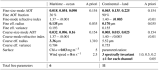
Table 2 contains details about each scene type. Both consist of a bimodal aerosol size distribution, partitioned into fine and coarse size modes with identical, spectrally invariant, complex refractive index (as is the case for the maritime (Lanai, Hawaii) and continental (Washington, DC) aerosol models in Dubovik et al., 2002). Partitioning between size modes is done in terms of the AOT (555 nm) fraction of the fine mode. Thus, the maritime scene is dominated by aerosols in the coarse size mode, while the continental scene is dominated by aerosols in the fine size mode, and the total aerosol load (AOT) for the scene is simply the sum of the fine- and coarse-mode loads.
The ocean surface reflectance was parameterized to represent a moderate Chl a load (a proxy for phytoplankton concentration that drives ocean reflectance) and specular reflectance of a surface roughened by a wind speed of 8 m s−1, after the model in Chowdhary et al. (2012). The land surface was parameterized using observations from a low-altitude aircraft scanner described in Knobelspiesse et al. (2008) as a model. This used the “Ross–Li” surface BRDF parameterization method (Lucht et al., 2000) for measurements of recently plowed agricultural fields near the US Department of Energy's Southern Great Plains site in Lamont, Oklahoma, USA. Both scene types used a single parameter to represent the BPDF with an angular dependence similar to Fresnel reflectance (for an example see Waquet et al., 2009).
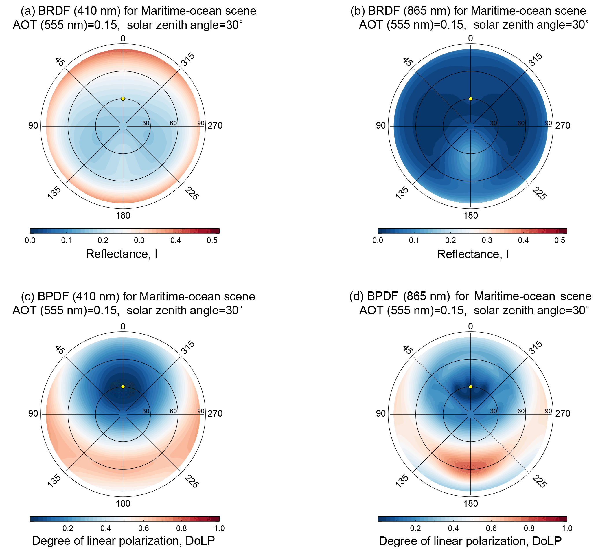
Figure 5Sample radiative transfer (RT) software output, for the maritime-ocean scene described in Table 2 for a moderate aerosol load of AOT (555 nm) = 0.15. The top row is the BRDF for the ocean and atmosphere scene at 410 nm (a) and 865 nm (b), while the bottom row is the same for the BPDF (expressed at DoLP). Like Fig. 2, view zenith angle (θv) is indicated in the radial coordinate dimension, while the relative angle between solar and view azimuth () is in the angular dimension, where a value of 0∘ is aligned with the solar azimuth angle. Note the significant differences between each BRDF or BPDF, which indicates the structure necessary for parameter retrieval, and the potential importance of appropriate sampling of the BRDF and or BPDF to maximize the information in such a retrieval.
The RT model was used to compute the simulated measurement vector y and its perturbation sensitivity as expressed in the Jacobian matrix, K. Perturbations (free parameters in a retrieval) were performed for 6 parameters for the maritime scene and 10 for the continental scene. The difference is due to the larger number of parameters needed to describe the land surface scene, including a spectrally variable parameter describing isotropic surface reflectance. Essentially, an additional parameter is needed for each spectral channel over land. Four parameters are used to describe aerosols in both types of scenes. For the maritime scene, free parameters are the fine-size-mode AOT, fine-size-mode effective radius, coarse-size-mode AOT and coarse-size-mode effective radius. For the continental scene (dominated by fine-size-mode aerosols), free parameters are the fine-size-mode AOT, fine-size-mode effective radius, fine-size-mode imaginary refractive index and coarse-size-mode AOT. In both cases, these are fewer parameters than the full set needed to describe the scene, as well as an acknowledgement of the underdetermined nature of a retrieval with these instrument configurations. In practice, a retrieval would involve the use of aerosol models or some other means of connecting parameters a priori to constrain the search in parameter space. For IC assessment, it is important to select a parameter space of realistically retrievable conditions, which is why we have limited the number of perturbations. Since we compare the information contained in different designs in a relative sense, we are less sensitive to the details of our choices of parameter space as long as they are broadly feasible for all our designs.
Figure 5 is a sample of the RT software output, where the BRDF of the maritime-ocean scene with a moderate aerosol load (AOT (555 nm) = 0.15) is shown in the top row for 410 nm (left) and 865 nm (right). The BPDF (in DoLP) is in the lower row. Note that the differences between each plot could contain information about the scene, as well as structure contained within each BRDF. Large amounts of structure (such as in the BPDF at 865 nm) could mean that there is sensitivity to the distribution of observations throughout the BPDF. To know for sure, we must place these results in the context of IC assessment.
3.4 Information content assessment
After completing the steps described above, IC assessment is performed by calculating the retrieval error covariance matrix, , and DFS using the scene Jacobian matrix K that has been subset appropriately for the instrument design. We must also create the observation error covariance matrix, Sϵ, and the a priori error covariance matrix, Sa.
As stated above, Sϵ describes measurement uncertainty, where each diagonal element of the matrix is the square of the individual uncertainty of an observation at the corresponding wavelength, view angle and polarization component. This includes both random and systematic (such as those related to calibration) uncertainties. Off-diagonal elements of the matrix represent the correlation between pairs of measurements, which we assumed for these cases is zero, meaning there are no measurement errors that would simultaneously impact multiple detectors. We expect this to be the case for observations made both by small satellites in formation and by instruments such as MISR, which have independent cameras for each viewing angle. Thus, Sϵ was chosen to be a diagonal matrix, with elements corresponding to I having an uncertainty of 3 %, and those corresponding to DoLP and uncertainty of 0.5 %. These values correspond to reasonable radiometric uncertainties for characterized orbital instruments (such as Eplee et al., 2012) and to desired polarimetric uncertainties cited for most future polarimetric instrument designs (Kokhanovsky et al., 2015).
Sa expresses our knowledge of state space prior to making an observation. In the context of the illustration in Fig. 4, this is the range of state (parameter) space in which a reasonable retrieval solution could reside based on our prior knowledge of the system. Our Sa was filled with squared a priori values shown in Table 2, which are based upon the same Dubovik et al. (2002) dataset as the aerosol models themselves. Like Sϵ, we assume no a priori correlation between parameters, and so Sa is diagonal.
Our IC assessment involves the calculation of many (more than 100 for each scene and instrument configuration) retrieval error covariance matrices, , and the corresponding averaging kernel matrices, A, correlation matrices and DFS. We consider eight architectures (the nine-view multi-angle instrument plus formations of three through nine single-view instruments), for six types of scenes (one maritime, one continental, at three AOT values each), for both radiometric and polarimetric sensors. In the case of the maritime-ocean scene, is a 6 × 6 matrix, while for the continental-land scene it is 10 × 10, meaning an iterative retrieval for those cases would have 6 and 10 free parameters, respectively.
Because of the scale of our IC assessment results, we present a subset that illustrate the overall outcome in light of our goal to compare observations by formations of single-view instruments to a multi-angle instrument. We start by comparing the DFS (Sect. 4.1) for different instruments and scenes as an overall metric of IC. Next, we assess the uncertainty for two aerosol parameters: the AOT (Sect. 4.2) and the fine-size-mode effective radius (Sect. 4.3). These were chosen because they were free parameters in all simulated scene types and because they are common to many aerosol retrievals. Section 4.4 describes the results in terms of the diagonals of the averaging kernel matrices, while in Sect. 4.5 we investigate the retrieved parameter correlation, which is not expressed in either the DFS or the individual parameter uncertainties.
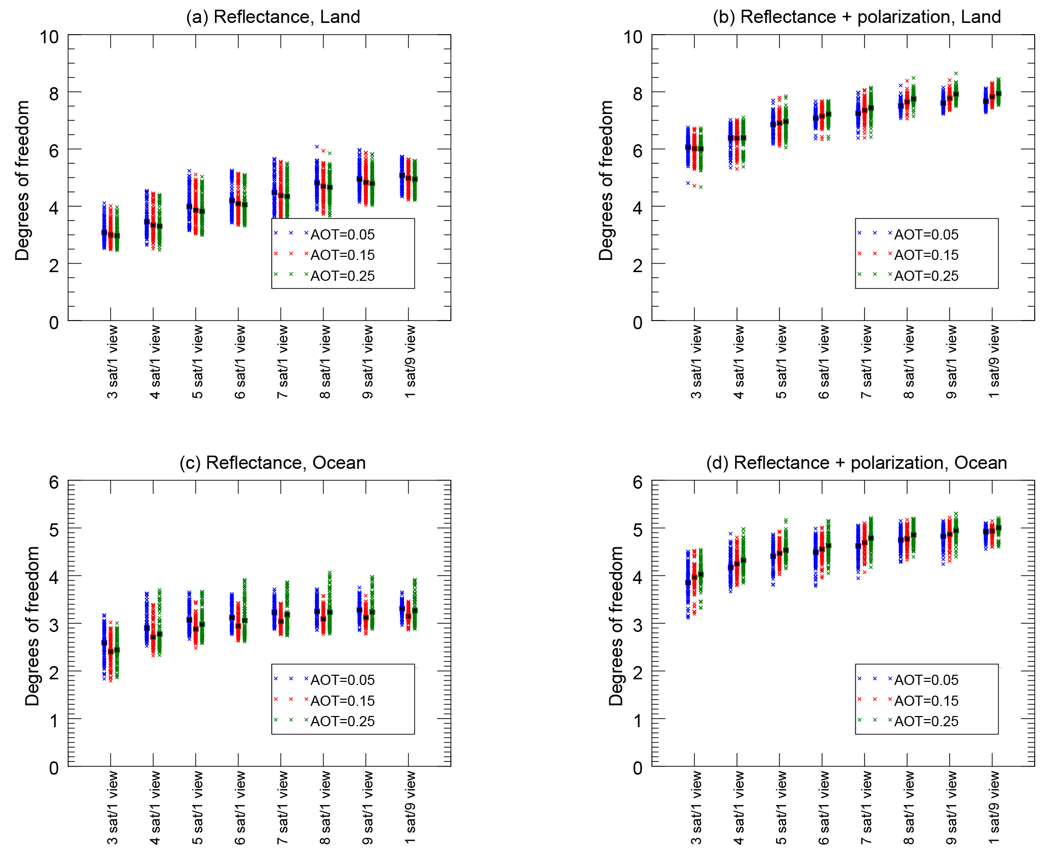
Figure 6The degrees of freedom for signal (DFS, described in Sect. 2.2) are plotted for continental aerosols over land (a, b), maritime aerosols over ocean (c, d) for instruments using reflectance alone (a, c) and reflectance plus DoLP (b, d). The simulated aerosol load is indicated by color and position, where total AOT (555 nm) equal to 0.05 is blue (left), AOT (555 nm) equal to 0.15 is red (center) and AOT (555 nm) equal to 0.25 is green (right). The number of single-view satellites is indicated along the abscissa, with the exception of the nine-view “multi-angle” instrument at the far right of each plot. The ordinate axis is the DFS, with a range representative of the theoretical maximum for that retrieval. The maximum DFS is equal to the number of free parameters (see Table 2) and is larger over land than over the ocean because of the larger number of parameters required to describe land surface reflectance. Thus, DFS indicates ability to retrieve both aerosol and surface parameters simultaneously.
4.1 Degrees of freedom for signal
As described in Sect. 2.2, the DFS is the trace of the averaging kernel matrix and therefore represents the overall capability of a measurement system. Capability, in this sense, is combined for parameters of interest to us (descriptive of aerosols) and those required to constrain surface reflectance. Figure 6 presents the DFS for each simulated scene and instrument configuration. In each plot, instrument configuration is expressed along the abscissa, and the DFS on the ordinate axis. Instruments using reflectance alone are indicated in the two plots at left, while those using reflectance and DoLP are at right. Aerosol retrievals over land are in the top row of figures, those over oceans are in the bottom row. Scene AOT is indicated by color and relative position within each plot (AOT = 0.05 in blue, left; AOT = 0.15 in red, center; AOT = 0.25 in green, right). The vertical spread of DFS for each configuration and scene represents the impacts of observation geometry variability among the predicted orbits. Black squares indicate the mean value of each group.
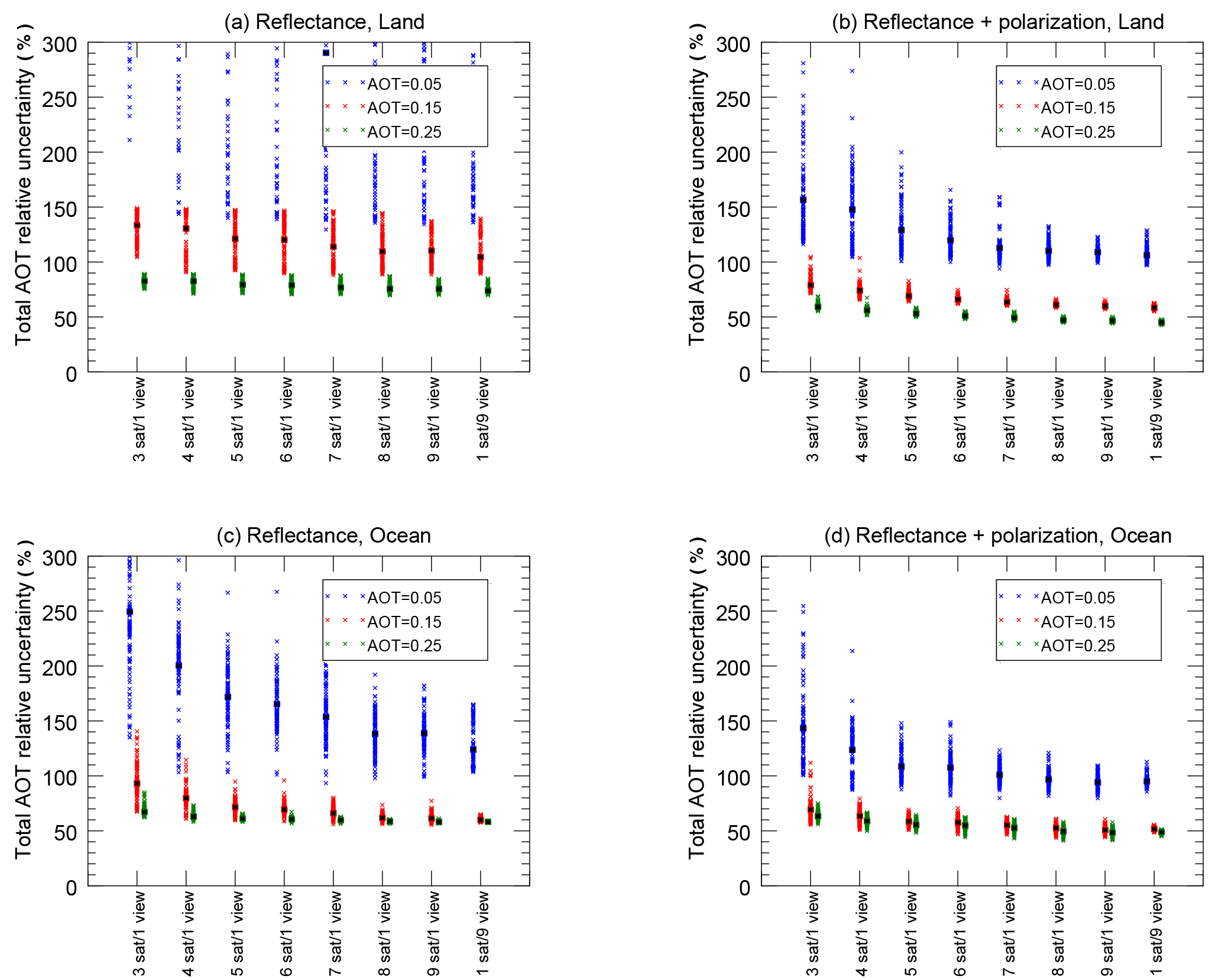
Figure 7Aerosol optical thickness (AOT) relative uncertainty at 555 nm is plotted for continental aerosols over land (a, b), maritime aerosols over ocean (c, d) for instruments using reflectance alone (a, c) and reflectance plus DoLP (b, d). The simulated aerosol load is indicated by color and position, where AOT (555 nm) equal to 0.05 is blue (left), AOT (555 nm) equal to 0.15 is red (center) and AOT (555 nm) equal to 0.25 is green (right). The number of single-view satellites is indicated along the abscissa, with the exception of the nine-view “multi-angle” single instrument at the far right. The ordinate axis is the relative uncertainty of the total (fine- and coarse-size-mode) AOT.
Regardless of scene type, all plots show a gentle increase in DFS as the number of satellites in each configuration are increased. DFS for the nine-satellite configuration and the multi-angle satellite with nine viewing angles are nearly indistinguishable, with differences in the mean values well within the variability range due to geometric differences in the orbit. This indicates that the capability of a measurement system, at least as expressed by the DFS, is primarily governed by the number of viewing angles, but not how those views are distributed within the BRDF or BPDF (although views from both the multi-angle satellite and the small satellites flying in formation are widely distributed throughout the BRDF or BPDF). Furthermore, this figure shows that the number of view angles gradually increases the DFS, such that a seven- or eight-satellite configuration is nearly as capable as the nine-satellite configuration or the nine-view multi-angle satellite configuration. For reflectance-only scenes over the ocean, in fact, the DFS tends to level off after five or six satellites, indicating diminishing returns with more angles. Polarimetric ocean and both reflectance-only and polarimetric land scenes benefit from additional viewing angles, although the DFS increase becomes more gradual.
A subtle difference between the single-view satellite configurations and the multi-angle instrument is present for the ocean case utilizing reflectance and polarization. In this case, the range of DFS values is slightly larger for the former compared to the latter. This means that, over the course of an orbit, there is a greater variability in the DFS for observations, although the mean uncertainty remains the same. In terms of ability to create global aerosol statistics, this difference may be irrelevant, but a study with a full OSSE may help identify whether there is a systematic geographical difference of relevance to the global aerosol distribution.
As expected, instrument configurations that utilize polarization have greater DFS, since they have access to more information. In fact, polarimetric observations over the ocean have a DFS of nearly 5, almost the theoretical limit (6) for that type of retrieval. We also do not see a large influence of the simulated AOT on the DFS. Since ability to retrieve aerosol optical properties depends on the aerosol load itself (Knobelspiesse et al., 2012), this probably means that the uniform DFS is expressing the transition between strong surface parameter capability when the aerosol load is low, which decreases with a corresponding increase in aerosol parameter capability as the aerosol load increases. We will find further support for this below.
4.2 Aerosol optical thickness
The AOT, as a measure of aerosol load, is one of the primary parameters retrieved from an instrument system. Our analysis expects the retrieval algorithm to independently determine the fine- and coarse-size-mode properties, including the individual mode optical thickness. The total AOT is a simple summation, so the uncertainty in its retrieval can be easily computed via Eq. (4). This is shown in Fig. 7 as a relative (to the simulation AOT) uncertainty. Like Fig. 6, this four-panel figure shows retrievals over land at top, over ocean at bottom, with reflectance only at left and reflectance with DoLP at right. Instrument configuration is the abscissa, and relative uncertainty for the total AOT is the ordinate axis. Simulations with a total AOT of 0.05 are in blue, 0.15 in red and 0.25 in green. We use 555 nm as the reference wavelength for AOT. At other wavelengths the AOT may be different, depending on aerosol properties.
Unlike, Fig. 6, however, the AOT relative uncertainty is strongly dependent upon the simulated AOT value itself. This is to be expected, as there is naturally more capability to determine aerosol optical properties if there are more aerosols present to affect the scene. In fact, relative uncertainty for AOT is greater than 100 % for nearly all instrument configurations for simulated scenes with an optical depth of 0.05. Considering that the global mean value of AOT is probably 3 or 4 times larger (Remer et al., 2008), this result shows an acceptable lower limit of aerosol detectability. Another striking characteristic of these results is that the number of viewing angles does not dramatically improve the relative AOT uncertainty, except for the lowest optical depths. Relative uncertainty seems to reach a minima as the number of viewing angles and the simulated AOT increase. An interpretation of this could be that AOT is expressed smoothly and uniformly throughout the BRDF, and increasing the number of viewing angles does not add to the information about AOT in the overall measurement. Echoing other analyses, polarization improves the AOT uncertainty, especially over land (Hasekamp, 2010; Hasekamp and Landgraf, 2007; Knobelspiesse et al., 2012).
These results support our hypothesis that single-view satellites in formation flight are equally capable as multi-angle observations on an individual satellite, provided that the number of viewing angles are the same. Furthermore, loss of one or more single-view satellites does not contribute much to an increase in uncertainty.
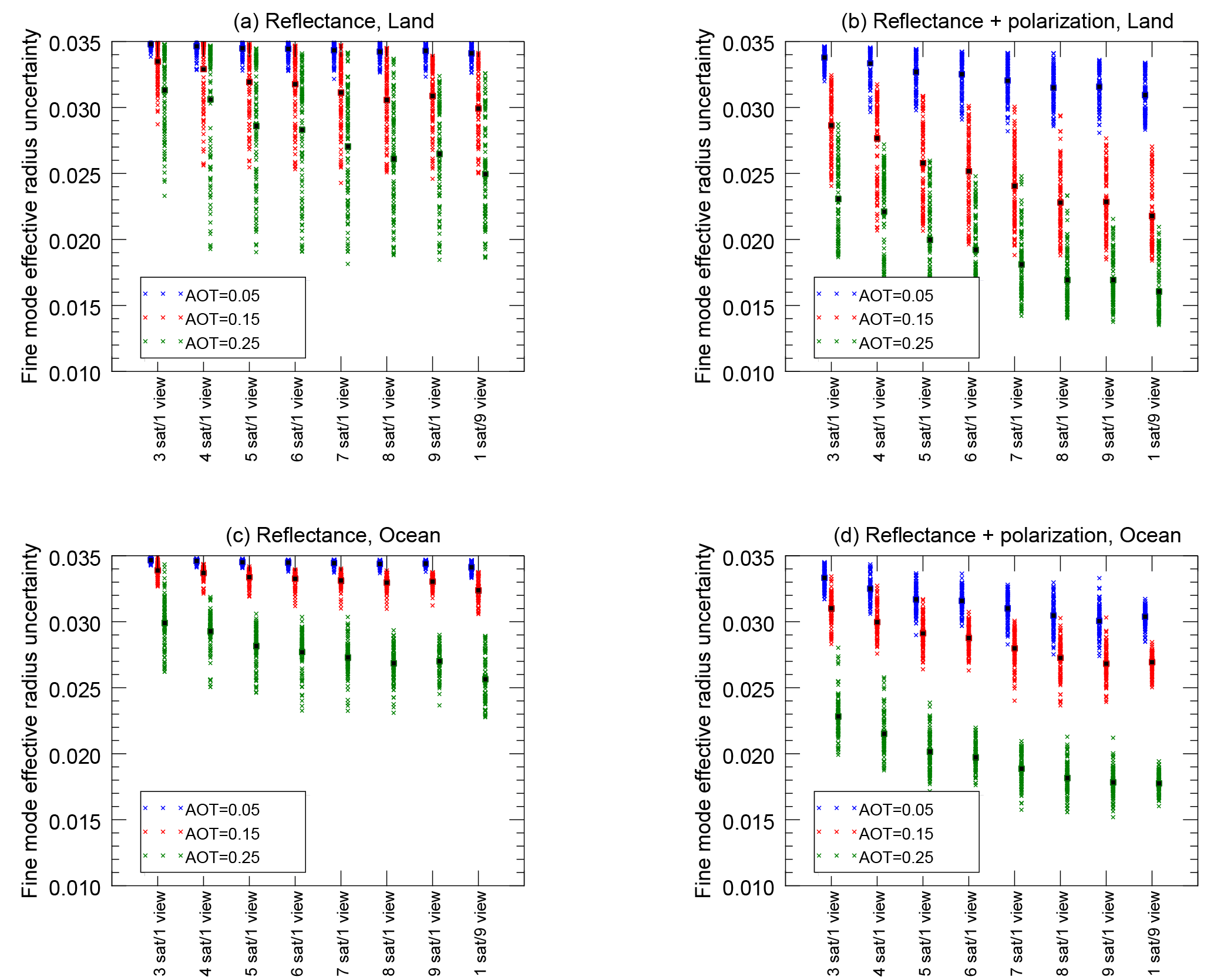
Figure 8Uncertainty in the effective radius for the fine aerosol size mode is plotted for continental aerosols over land (a, b), maritime aerosols over ocean (c, d) for instruments using reflectance alone (a, c) and reflectance plus DoLP (b, d). The simulated aerosol load is indicated by color and position, where AOT (555 nm) equal to 0.05 is blue (left), AOT (555 nm) equal to 0.15 is red (center) and AOT (555 nm) equal to 0.25 is green (right). The number satellites and view angles is indicated along the abscissa. The ordinate axis is the uncertainty for the fine-size-mode effective radius from the square root of the corresponding element on the diagonal of . The maximum value of each ordinate axis is the a priori uncertainty specified in Sa, the theoretically largest value possible. Results close to this indicate no sensitivity. Also, note that the contribution of the fine size mode to the total aerosol extinction was different for the simulations over land and ocean. Over land, the fine mode contributed 90 % to the total aerosol optical depth, while over ocean it was 36 % (see Table 2).
4.3 Fine-size-mode effective radius
The uncertainty of determining the effective radius (one of two parameters defining size distribution) of the fine (small) aerosol size mode is plotted in Fig. 8. Like Figs. 6 and 7, this four-panel figure shows retrievals over land at top, over ocean at bottom, with reflectance only at left and reflectance and DoLP at right, while instrument configuration is the abscissa, and relative uncertainty for the total AOT is the ordinate axis. The maximum value of the ordinate axis is the a priori uncertainty, which is the theoretical maximum (least certain) value for uncertainty for a parameter in Eq. (2). Results close to this value indicate that the measurement has provided no additional information about that parameter compared to what was known prior to measurement.
We chose to display the fine-mode effective radius because it is a parameter that was shared between both types of scenes, although the fine size mode contributed different amounts to the total AOT in each scene. For ocean scenes, the fine mode contributed 36 % to the total AOT, while over land the contribution was 90 %. This means the fine size mode had a stronger role modifying the observed BRDF and BPDF over land than over ocean, contributing to the lower uncertainties for the former compared to the latter. Otherwise, the uncertainty for the fine-mode effective radius follows many of the same patterns as the AOT. For the lowest simulation AOT (0.05), uncertainty was close to the a priori value for the reflectance only instruments, but slightly better for instruments that used polarization. Additional angles do help a bit more than was the case for AOT, although the improvement is gradual. Furthermore, we found no significant differences between the nine satellites in formation flight compared to a multi-angle satellite with nine views.
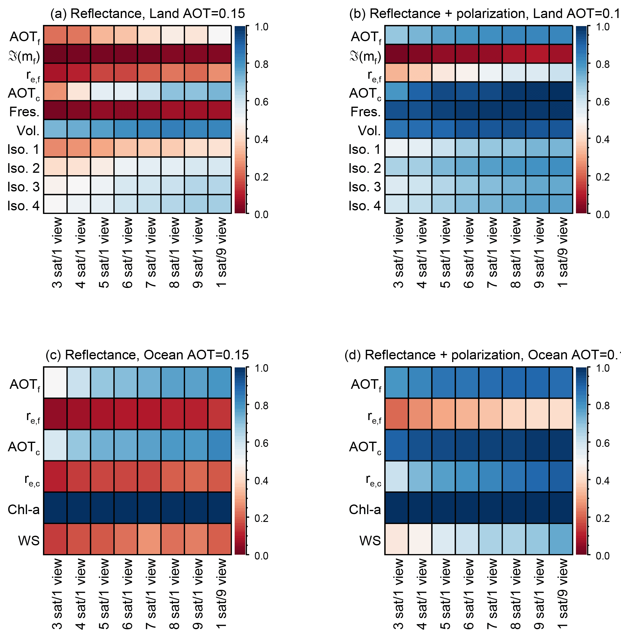
Figure 9Diagonal values for the mean averaging kernel matrices, A, for land scenes (a, b), ocean scenes (c, d) using observations of reflectance only (a, c) and DoLP with reflectance (b, d). These values roughly represent what fraction of a retrieved parameter is due to the observations and not a priori values. Results are shown for each satellite configuration (abscissa), while the ordinate axis has the results for each parameter described in Table 2. For the land scene, these parameters are, from the top, fine-size-mode AOT, imaginary component of the refractive index of the fine size mode, effective radius for the fine size mode, coarse-size-mode AOT, fresnel (polarized) surface reflectance coefficient, volumetric (BRDF shape) surface reflectance coefficient and isotropic reflectance coefficients for each band, at 410, 555, 865 and 2250 nm. For the ocean scene, these parameters are, from the top: fine-size-mode AOT, effective radius for the fine size mode, coarse-size-mode AOT, effective radius for the coarse size mode, ocean body Chl a content and ocean surface wind speed. The sum of each column is the DFS for each instrument configuration as shown in Fig. 6. This figure therefore displays how those DFS values are partitioned among the retrieval parameters.
4.4 Averaging kernel matrix
The averaging kernel matrix (A) diagonals for different scene types and observation configurations are illustrated in Fig. 9. As described in Sect. 2.2, the diagonals of the averaging kernel matrix represent how independent retrieved parameters will be from the a priori matrix. Thus, a diagonal value close to 1 indicates significant information about that parameter in the observations or at least that there is significantly more information than defined in the a priori matrix. The DFS in Fig. 6 is the sum of these values (in other words, the trace of A). This figure thus describes how the DFS are shared among the parameters, an important distinction.
The most obvious inference from Fig. 9 is that values for a parameter are generally equivalent across instrument configurations, with limited improvement as the number of viewing angles increases. Some parameters have high values in nearly all cases – examples include Chl a for ocean scenes or the Fresnel polarimetric surface coefficient for land scenes with polarimetrically sensitive instruments. In these cases, a priori values were set to be large so that they did not impact results for aerosol-related parameters. Retrieval uncertainties for Chl a, at least, are not much larger than typical values (McClain, 2009), which is reasonable given the low simulated Chl a value and lack of ocean color-specific channels in our hypothetical instruments. Some parameters have very low values, such as, for land scenes, the imaginary part of the fine-size-mode refractive index (associated with aerosol absorption) or the Fresnel coefficient for instruments without polarization sensitivity. These parameters show little improvement with additional view angles. Many parameters are in between these extremes, and these show the most sensitivity to an increase in the number of view angles. In any case, this provides the means to understand the partitioning of degrees of freedom for a given system. For example, a nine-view, reflectance-only ocean observation has a DFS of roughly 3, which is primarily driven by Chl a (ocean body reflectance), and the AOT of both aerosol size modes.
These results represent the mean value of A diagonals across all orbits for an AOT (555 nm) = 0.15. For brevity, we have not included results for simulations for smaller and larger AOT since the general patterns remain. As expected, at low AOT values for surface parameters increase while aerosol parameters decrease. It is the opposite for larger AOT, as the increase in aerosol load increases the impact of aerosols on observations as the expense of surface reflection.
Finally, what is clear from Fig. 9 is that configuration differences between the nine satellites flying in formation and the multi-angle single-view satellite have an imperceptible impact on A.
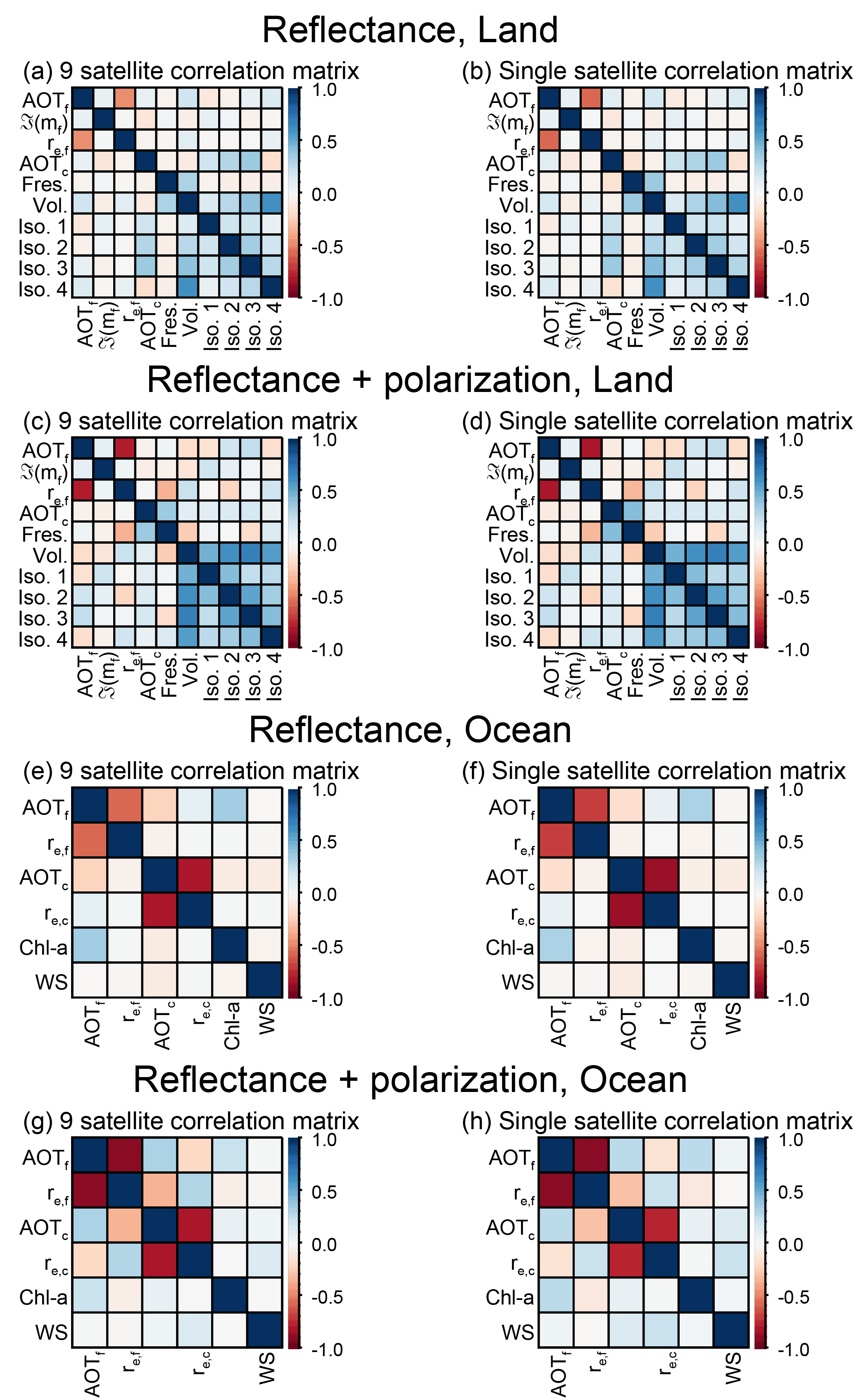
Figure 10Correlation matrixes for scenes with the medium simulated optical depth (AOT (555 nm) = 0.15) are shown for scenes over land (a, b, c, d), over ocean (e, f, g, h), for retrievals using reflectance alone (a, b, e, f) and reflectance and DoLP (c, d, g, h). Matrices represent the average for all simulations throughout the orbit for that configuration, although only simulations with nine view angles (nine satellites in formation and nine-view multi-angle satellite) are shown.
4.5 Correlation matrix
Figure 10 contains the retrieval error correlation matrix, (Eq. 6), for the configurations of the nine-view-angle instrument. As described in Sect. 2.2, large off-diagonal values indicate a smaller volume in retrieval state space, an indication of higher IC for that pair of parameters. We can see this in the slight increase in correlation (or anticorrelation) for retrievals utilizing polarization, an expected improvement with additional knowledge. All scenes demonstrate a strong anticorrelation between AOT and the effective radius of the same size mode. Physically, these parameters should be uncorrelated, since effective radius is an intrinsic optical parameter, while AOT is an extrinsic parameter expressing total column extinction. Thus, our assumption of no correlation between these parameters in the a priori error covariance matrix (Sa in Eq. 2) is probably valid. This would thus indicate that the source of the anticorrelation is the nature of parameter space expressed in the Jacobians. In practice it would not indicate a relationship in the retrievals of the parameters, but if one retrieved parameter were wrong, we could expect the other parameter to also be wrong (but in the direction of the opposite sign).
Most importantly, these matrices are nearly identical for the nine satellites flying in formation flight and the nine-view multi-angle instrument. This is further support for the hypothesis that satellites in formation flight are equally capable of retrieving aerosol parameters as multi-angle instruments.
Our central hypothesis is that aerosol remote sensing is performed equally well by the geometric distribution of observations by small satellites flying in formation and multi-angle views on a single satellite. The main difference between the two types of observations is that multi-angle views on a single satellite are restricted to a single azimuth plane, while small satellites flying in formation observe at a variety of azimuth angles. Such systems therefore sample the BRDF or BPDF in different ways. To test this hypothesis, we have generated a variety of observation formations using a systems engineering orbital model constrained to feasible satellite bus configurations. The geometries of these formations where then used as inputs to an IC analysis, which determines geophysical parameter retrieval capability. This capability was tested for the aggregate of the observation formations for a variety of realistic atmospheric aerosol scenes over land and ocean. These tests were performed for formations of between three and nine satellites to compare to a multi-angle satellite with nine views. All instruments were simulated with identical spectral and measurement uncertainty characteristics. Details about the limitations of our IC technique are discussed in Sect. 2.2.
The IC analysis reveals that there is no difference between the capability of multi-angle satellite instruments on a single platform compared to an equal number of views from satellites flying in formation. This equivalence is maintained for a variety of aerosol classes, quantities and scene types (over land or over ocean). The primary factor affecting capability (other than spectral characteristics and measurement uncertainty, which we did not vary) is the number of viewing angles in a observation, and not their distribution throughout the BRDF and BPDF. This can be explained by the smooth nature of TOA BRDF and BPDF (see Fig. 5), meaning that constraining observations to a particular plane in the BRDF or BPDF (as is the case with multi-angle instruments) yields no advantages or disadvantages.
We also found that the IC improves only incrementally as the number of viewing angles increases. For some situations and parameters, additional viewing angles provide no improvement after a half dozen or so, while others (typically those for which the observation system has marginal overall IC) do show improvements that eventually level off with many view angles. This is slightly lower than the conclusions of Hasekamp (2010), who found that 16 viewing angles are sufficient for retrieval of most aerosol optical properties, and that the capability (for aerosols) with more viewing angles is constrained by the angle to angle measurement correlation present in most multi-angle imaging systems. While we do not account for observation correlation (unlikely in measurement systems such as ours) the difference is probably due to our more constrained parameter space.
Further investigation into the value of aerosol remote sensing with small satellites in formation would need to address topics we could not consider in this IC study. We assumed that the measurement uncertainties are identical for different designs, and this may not be the case. Small satellites flying in formation may have differences in how they are calibrated compared to single platform spacecraft, and the relative differences between satellites may be more difficult to characterize than the differences between view angles in a single spacecraft. These differences would pertain to specific designs and not be generally applicable as in this paper. Successful co-registration of multi-angle views between designs may vary, but again this is a design-specific metric. Another topic we could not consider was the impact of instrument swath and coverage. Obviously, greater coverage is desirable, but the impact of this in determining climate-relevant information requires the use of a full OSSE. Coupling orbit geometries from the systems engineering model to simulated observations from the nature run of an OSSE would provide the means to more directly assess the ability to observe parameters of relevance to climate.
In addition to our central hypothesis, this analysis reveals useful general details about the IC of multi-angle and multi-angle polarimetric observations. As illustrated in Fig. 6, a multi-angle observation over land has roughly 4 DFS, while polarimetric observations (with a DoLP accuracy of 0.005) add roughly 3 more DFS to this. Over the ocean, there are roughly 3 DFS, and adding polarization about 1.5 DFS to that. Aerosol retrievals require parameterization of the surface reflectance, so these DFS are partitioned between aerosol-relevant parameters and surface-relevant parameters, as shown in Fig. 9. The scene aerosol load (total AOT) drives this partitioning, such that large AOT increases DFS in aerosol parameters at the expense of surface parameters, and vice versa for small AOT. The impact of this can be seen in the individual uncertainty estimates for total AOT (Fig. 7) and fine-size-mode effective radius (Fig. 8), which show a distinct improvement with increasing AOT. These results mirror other sensitivity studies (such as Hasekamp, 2010; Hasekamp and Landgraf, 2007; Hasekamp et al., 2011; Knobelspiesse et al., 2012) and supports the notion that our methodology is sound.
To date, multi-angle remote sensing of aerosols have only been performed with instruments that make all of their observations on a single spacecraft. Ongoing technological development means that coordinated observations by formations of satellites are becoming a reality. We have demonstrated that the information contained in such observations would be equivalent to a single multi-angle instrument for aerosol remote sensing. While many technical and scientific matters must still be resolved, this provides an opportunity, as these formations may have engineering, cost or other advantages. They may, for example, be more resilient. Our results indicate that the loss of one or more individual satellites does not dramatically impact the IC in the observation, providing for an opportunity to replace lost satellites, ultimately improving observation continuity. Where there remains many aspects of such observations to explore, they hold promise for the future of aerosol remote sensing.
Raw data will be provided by the corresponding author upon request.
KK performed the information content analysis with input from the systems engineering tool developed by author SN. Concept, experiment design and manuscript preparation were joint efforts of both authors.
The authors declare that they have no conflict of interest.
The first author was supported in this research by an award from the NASA New
(Early Career) Investigator Program in Earth Science, NNH13ZDA001N-NIP,
managed by Ming-Ying Wei and Lin Chambers. The research was conducted at both
the NASA Ames Research Center in Moffett Field, California, and the NASA
Goddard Space Flight Center in Greenbelt, Maryland. The doubling and adding
radiative transfer code used in this work was developed at the NASA Goddard
Institute for Space Studies, with recent updates by Brian Cairns and Jacek
Chowdhary at that institution.
Edited by: Sebastian Schmidt
Reviewed by: Feng Xu and Odele Coddington
Blackwell, W. J.: The MicroMAS and MiRaTA CubeSat atmospheric profiling missions, in: 2015 IEEE MTT-S International Microwave Symposium, Phoenix, AZ, USA, 17–22 May 2015, IEEE, 1–3, 2015. a
Cairns, B., Russell, E. E., LaVeigne, J. D., and Tennant, P. M.: Research scanning polarimeter and airborne usage for remote sensing of aerosols, Proc. SPIE, 5158, 33–44, 2003. a
Chowdhary, J., Cairns, B., Waquet, F., Knobelspiesse, K., Ottaviani, M., Redemann, J., Travis, L., and Mishchenko, M.: Sensitivity of multiangle, multispectral polarimetric remote sensing over open oceans to water-leaving radiance: Analyses of RSP data acquired during the MILAGRO campaign, Remote Sens. Environ., 118, 284–308, 2012. a
Coddington, O., Pilewskie, P., and Vukicevic, T.: The Shannon information content of hyperspectral shortwave cloud albedo measurements: Quantification and practical applications, J. Geophys. Res., 117, D04205, https://doi.org/10.1029/2011JD016771, 2012. a
Coddington, O., Pilewskie, P., Schmidt, K. S., McBride, P. J., and Vukicevic, T.: Characterizing a New Surface-Based Shortwave Cloud Retrieval Technique, Based on Transmitted Radiance for Soil and Vegetated Surface Types, Atmosphere, 4, 48–71, https://doi.org/10.3390/atmos4010048, 2013. a
Coddington, O., Vukicevic, T., Schmidt, K., and Platnick, S.: Characterizing the information content of cloud thermodynamic phase retrievals from the notional PACE OCI shortwave reflectance measurements, J. Geophys. Res.-Atmos., 122, 8079–8100, 2017. a
Colarco, P., da Silva, A., Chin, M., and Diehl, T.: Online simulations of global aerosol distributions in the NASA GEOS-4 model and comparisons to satellite and ground-based aerosol optical depth, J. Geophys. Res., 115, D14207, https://doi.org/10.1029/2009JD012820, 2010. a
de Haan, J., Bosma, P., and Hovenier, J.: The adding method for multiple scattering calculations of polarized light, Astron. Astrophys., 183, 371–391, 1987. a
Diner, D., Beckert, J., Reilly, T., Bruegge, C., Conel, J., Kahn, R., Martonchik, J., Ackerman, T., Davies, R., Gerstl, S., Gordon, H., Muller, J., Myneni, R., Sellers, P., Pinty, B., and Verstraete, M.: Multi-angle Imaging SpectroRadiometer (MISR) instrument description and experiment overview, IEEE T. Geosci. Remote, 36, 1072–1087, 1998. a
Dubovik, O., Holben, B., Eck, T., Smirnov, A., Kaufman, Y., King, M., Tanré, D., and Slutsker, I.: Variability of absorption and optical properties of key aerosol types observed in worldwide locations, J. Atmos. Sci., 59, 590–608, 2002. a, b, c
Dubovik, O., Herman, M., Holdak, A., Lapyonok, T., Tanré, D., Deuzé, J. L., Ducos, F., Sinyuk, A., and Lopatin, A.: Statistically optimized inversion algorithm for enhanced retrieval of aerosol properties from spectral multi-angle polarimetric satellite observations, Atmos. Meas. Tech., 4, 975–1018, https://doi.org/10.5194/amt-4-975-2011, 2011. a
Eplee, R. E., Meister, G., Patt, F. S., Barnes, R. A., Bailey, S. W., Franz, B. A., and McClain, C. R.: On-orbit calibration of SeaWiFS, Appl. Optics, 51, 8702–8730, 2012. a
Fougnie, B., Bracco, G., Lafrance, B., Ruffel, C., Hagolle, O., and Tinel, C.: PARASOL in-flight calibration and performance, Appl. Optics, 46, 5435–5451, 2007. a, b
Friedl, M. A., Sulla-Menashe, D., Tan, B., Schneider, A., Ramankutty, N., Sibley, A., and Huang, X.: MODIS Collection 5 global land cover: Algorithm refinements and characterization of new datasets, Remote Sens. Environ., 114, 168–182, 2010. a
Gatebe, C. K. and King, M. D.: Airborne spectral {BRDF} of various surface types (ocean, vegetation, snow, desert, wetlands, cloud decks, smoke layers) for remote sensing applications, Remote Sens. Environ., 179, 131–148, 2016. a
Hansen, J. and Travis, L.: Light scattering in planetary atmospheres, Space Sci. Rev., 16, 527–610, 1974. a
Hasekamp, O. P.: Capability of multi-viewing-angle photo-polarimetric measurements for the simultaneous retrieval of aerosol and cloud properties, Atmos. Meas. Tech., 3, 839–851, https://doi.org/10.5194/amt-3-839-2010, 2010. a, b, c
Hasekamp, O. and Landgraf, J.: Retrieval of aerosol properties over land surfaces: capabilities of multiple-viewing-angle intensity and polarization measurements, Appl. Optics, 46, 3332–3344, 2007. a, b, c, d
Hasekamp, O., Litvinov, P., and Butz, A.: Aerosol properties over the ocean from PARASOL multiangle photopolarimetric measurements, J. Geophys. Res., 116, D14204, https://doi.org/10.1029/2010JD015469, 2011. a, b
IPCC: Climate Change 2013 – The Physical Science Basis: Contribution of the Working Group I to the Fifth Assessment Report of the IPCC, Cambridge University Press, New York, NY, 2013. a
Kahn, R., Banerjee, P., and McDonald, D.: Sensitivity of multiangle imaging to natural mixtures of aerosols over ocean, J. Geophys. Res., 106, 18219–18238, 2001. a, b
Kahn, R., Gaitley, B., Martonchik, J., Diner, D., Crean, K., and Holben, B.: Multiangle Imaging Spectroradiometer (MISR) global aerosol optical depth validation based on 2 years of coincident Aerosol Robotic Network (AERONET) observations, J. Geophys. Res., 110, D10S04, https://doi.org/10.1029/2004JD004706, 2005. a
Knobelspiesse, K., Cairns, B., Schaaf, C., Schmid, B., and Román, M.: Surface BRDF estimation from an aircraft compared to MODIS and ground estimates at the Southern Great Plains site, J. Geophys. Res., 113, D20105, https://doi.org/10.1029/2008JD010062, 2008. a, b, c
Knobelspiesse, K., Cairns, B., Ottaviani, M., Ferrare, R., Hair, J., Hostetler, C., Obland, M., Rogers, R., Redemann, J., Shinozuka, Y., Clarke, A., Freitag, S., Howell, S., Kapustin, V., and McNaughton, C.: Combined retrievals of boreal forest fire aerosol properties with a polarimeter and lidar, Atmos. Chem. Phys., 11, 7045–7067, https://doi.org/10.5194/acp-11-7045-2011, 2011a. a
Knobelspiesse, K., Cairns, B., Redemann, J., Bergstrom, R. W., and Stohl, A.: Simultaneous retrieval of aerosol and cloud properties during the MILAGRO field campaign, Atmos. Chem. Phys., 11, 6245–6263, https://doi.org/10.5194/acp-11-6245-2011, 2011b. a
Knobelspiesse, K., Cairns, B., Mishchenko, M., Chowdhary, J., Tsigaridis, K., van Diedenhoven, B., Martin, W., Ottaviani, M., and Alexandrov, M.: Analysis of fine-mode aerosol retrieval capabilities by different passive remote sensing instrument designs, Opt. Express, 20, 21457–21484, 2012. a, b, c, d, e, f, g, h
Knobelspiesse, K., van Diedenhoven, B., Marshak, A., Dunagan, S., Holben, B., and Slutsker, I.: Cloud thermodynamic phase detection with polarimetrically sensitive passive sky radiometers, Atmos. Meas. Tech., 8, 1537–1554, https://doi.org/10.5194/amt-8-1537-2015, 2015. a
Kokhanovsky, A., Davis, A., Cairns, B., Dubovik, O., Hasekamp, O., Sano, I., Mukai, S., Rozanov, V., Litvinov, P., Lapyonok, T., Kolomiets, I., Oberemok, Y., Savenkov, S., Martin, W., Wasilewski, A., di Noia, A., Stap, A., Rietjens, J., Xu, F., Natraj, V., Duan, M., Cheng, T., and Munro, R.: Space-Based Remote Sensing of Atmospheric Aerosols: The Multi-Angle Spectro-Polarimetric Frontier, Earth-Sci. Rev., 145, 85–116, 2015. a, b
Lucht, W., Schaaf, C., and Strahler, A.: An algorithm for the retrieval of albedo from space using semiempirical BRDF models, IEEE T. Geosci. Remote, 38, 977–998, 2000. a
Marbach, T., Phillips, P., and Schlüssel, P.: 3MI: The Multi-Viewing Multi-Channel Multi-Polarization Imaging Mission of the EUMETSAT Polar System-Second Generation (EPS-SG) dedicated to aerosol characterization, AIP Conf. Proc., 1531, 344–347, 2013. a
McClain, C. R.: A decade of satellite ocean color observations, Annu. Rev. Mar. Sci., 1, 19–42, 2009. a
Mishchenko, M., Cairns, B., Hansen, J., Travis, L., Burg, R., Kaufman, Y., Vanderlei Martins, J., and Shettle, E.: Monitoring of aerosol forcing of climate from space: analysis of measurement requirements, J. Quant. Spectrosc. Ra., 88, 149–161, 2004. a
Nadal, F. and Breon, F.-M.: Parameterization of Surface Polarized Reflectance Derived from POLDER Spaceborne Measurements, IEEE T. Geosci. Remote, 37, 1709–1718, 1999. a
Nag, S., Gatebe, C. K., and de Weck, O.: Observing system simulations for small satellite formations estimating bidirectional reflectance, Int. J. Appl. Earth Obs., 43, 102–118, 2015. a, b, c
Nag, S., Gatebe, C. K., Miller, D. W., and de Weck, O. L.: Effect of satellite formations and imaging modes on global albedo estimation, Acta Astronaut., 126, 77–97, 2016. a, b, c, d, e, f, g, h
Nag, S., Gatebe, C. K., and Hilker, T.: Simulation of multiangular remote sensing products using small satellite formations, IEEE J. Sel. Top. Appl., 10, 638–653, 2017a. a, b, c
Nag, S., Hewagama, T., Georgiev, G. T., Pasquale, B., Aslam, S., and Gatebe, C. K.: Multispectral Snapshot Imagers Onboard Small Satellite Formations for Multi-Angular Remote Sensing, IEEE Sens. J., 17, 5252–5268, 2017b. a
Nag, S., Li, A. S., and Merrick, J. H.: Scheduling algorithms for rapid imaging using agile Cubesat constellations, Adv. Space Res., 61, 891–913, 2018. a
Nicodemus, F. E., Richmond, J. C., Hsia, J. J., Ginsberg, I. W., and Limperis, T.: Geometrical Considerations and Nomenclature for Reflectance, National Bureau of Standards, NBS monograph 160, 74 pp., 1977. a
O'Neill, N., Ignatov, A., Holben, B., and Eck, T.: The lognormal distribution as a reference for reporting aerosol optical depth statistics: Empirical tests using multi-year, multi-site AERONET sunphotometer data, Geophys. Res. Lett., 27, 3333–3336, 2000. a
Ottaviani, M., Cairns, B., Chowdhary, J., Van Diedenhoven, B., Knobelspiesse, K., Hostetler, C., Ferrare, R., Burton, S., Hair, J., Obland, M., and Rogers, R.: Polarimetric retrievals of surface and cirrus clouds properties in the region affected by the Deepwater Horizon oil spill, Remote Sens. Environ., 121, 389–403, 2012. a
Ottaviani, M., Knobelspiesse, K., Cairns, B., and Mishchenko, M.: Information content of aerosol retrievals in the sunglint region, Geophys. Res. Lett., 40, 631–634, 2013. a
Ottaviani, M., van Diedenhoven, B., and Cairns, B.: Photopolarimetric retrievals of snow properties, The Cryosphere, 9, 1933–1942, https://doi.org/10.5194/tc-9-1933-2015, 2015. a
Peralta, R., Nardell, C., Cairns, B., Russell, E., Travis, L., Mishchenko, M., Fafaul, B., and Hooker, R.: Aerosol polarimetry sensor for the Glory Mission, Proc. SPIE, 6786, 6786-1–6786-17, https://doi.org/10.1117/12.783307, 2007. a
Remer, L. A., Kaufman, Y., and Kleidman, R.: Comparison of Three Years of Terra and Aqua MODIS Aerosol Optical Thickness Over the Global Oceans, IEEE Geosci. Remote S., 3, 537–540, 2006. a
Remer, L. A., Kleidman, R. G., Levy, R. C., Kaufman, Y., Tanré, D., Mattoo, S., Martins, J. V., Ichoku, C., Koren, I., Yu, H., and Holben, B.: Global aerosol climatology from the MODIS satellite sensors, J. Geophys. Res., 113, D14S07, https://doi.org/10.1029/2007JD009661, 2008. a
Rodgers, C.: Inverse Methods for Atmospheric Sounding: Theory and Practice, World Scientific, Singapore, 2000. a, b
Ruf, C. S., Gleason, S., Jelenak, Z., Katzberg, S., Ridley, A., Rose, R., Scherrer, J., and Zavorotny, V.: The CYGNSS nanosatellite constellation hurricane mission, in: 2012 IEEE International Geoscience and Remote Sensing Symposium, Munich, Germany, 22–27 July 2012, IEEE, 214–216, 2012. a
Smith, G., Priestley, K., Loeb, N., Wielicki, B., Charlock, T., Minnis, P., Doelling, D., and Rutan, D.: Clouds and Earth Radiant Energy System (CERES), a review: Past, present and future, Adv. Space Res., 48, 254–263, 2011. a
Tanré, D., Bréon, F. M., Deuzé, J. L., Dubovik, O., Ducos, F., François, P., Goloub, P., Herman, M., Lifermann, A., and Waquet, F.: Remote sensing of aerosols by using polarized, directional and spectral measurements within the A-Train: the PARASOL mission, Atmos. Meas. Tech., 4, 1383–1395, https://doi.org/10.5194/amt-4-1383-2011, 2011. a
van Diedenhoven, B., Cairns, B., Geogdzhayev, I. V., Fridlind, A. M., Ackerman, A. S., Yang, P., and Baum, B. A.: Remote sensing of ice crystal asymmetry parameter using multi-directional polarization measurements – Part 1: Methodology and evaluation with simulated measurements, Atmos. Meas. Tech., 5, 2361–2374, https://doi.org/10.5194/amt-5-2361-2012, 2012. a
van Diedenhoven, B., Fridlind, A. M., Cairns, B., and Ackerman, A. S.: Variation of ice crystal size, shape, and asymmetry parameter in tops of tropical deep convective clouds, J. Geophys. Res.-Atmos., 119, 11809–11825, 2014. a
Vukicevic, T., Coddington, O., and Pilewskie, P.: Characterizing the retrieval of cloud properties from optical remote sensing, J. Geophys. Res., 115, D20211, https://doi.org/10.1029/2009JD012830, 2010. a
Wang, J., Xu, X., Ding, S., Zeng, J., Spurr, R., Liu, X., Chance, K., and Mishchenko, M.: A numerical testbed for remote sensing of aerosols, and its demonstration for evaluating retrieval synergy from a geostationary satellite constellation of GEO-CAPE and GOES-R, J. Quant. Spectrosc. Ra., 146, 510–528, 2014. a
Waquet, F., Cairns, B., Knobelspiesse, K., Chowdhary, J., Travis, L., Schmid, B., and Mishchenko, M.: Polarimetric remote sensing of aerosols over land, J. Geophys. Res., 114, D01206, https://doi.org/10.1029/2008JD010619, 2009. a
Wielicki, B. A., Barkstrom, B. R., Harrison, E. F., Lee III, R. B., Louis Smith, G., and Cooper, J. E.: Clouds and the Earth's Radiant Energy System (CERES): An earth observing system experiment, B. Am. Meteorol. Soc., 77, 853–868, 1996. a
Xu, X. and Wang, J.: Retrieval of aerosol microphysical properties from AERONET photopolarimetric measurements: 1. Information content analysis, J. Geophys. Res.-Atmos., 120, 7059–7078, 2015. a