the Creative Commons Attribution 4.0 License.
the Creative Commons Attribution 4.0 License.
 | 30 Aug 2019
Development and validation of a supervised machine learning radar Doppler spectra peak-finding algorithm
Heike Kalesse
Teresa Vogl
Cosmin Paduraru
Edward Luke
In many types of clouds, multiple hydrometeor populations can be present at the same time and height. Studying the evolution of these different hydrometeors in a time–height perspective can give valuable information on cloud particle composition and microphysical growth processes. However, as a prerequisite, the number of different hydrometeor types in a certain cloud volume needs to be quantified. This can be accomplished using cloud radar Doppler velocity spectra from profiling cloud radars if the different hydrometeor types have sufficiently different terminal fall velocities to produce individual Doppler spectrum peaks. Here we present a newly developed supervised machine learning radar Doppler spectra peak-finding algorithm (named PEAKO). In this approach, three adjustable parameters (spectrum smoothing span, prominence threshold, and minimum peak width at half-height) are varied to obtain the set of parameters which yields the best agreement of user-classified and machine-marked peaks. The algorithm was developed for Ka-band ARM zenith-pointing radar (KAZR) observations obtained in thick snowfall systems during the Atmospheric Radiation Measurement Program (ARM) mobile facility AMF2 deployment at Hyytiälä, Finland, during the Biogenic Aerosols – Effects on Clouds and Climate (BAECC) field campaign. The performance of PEAKO is evaluated by comparing its results to existing Doppler peak-finding algorithms. The new algorithm consistently identifies Doppler spectra peaks and outperforms other algorithms by reducing noise and increasing temporal and height consistency in detected features. In the future, the PEAKO algorithm will be adapted to other cloud radars and other types of clouds consisting of multiple hydrometeors in the same cloud volume.
- Article
(21776 KB) - Full-text XML
- BibTeX
- EndNote


Determining cloud composition in terms of hydrometeor populations is a nontrivial task in thick, cold precipitating clouds below 0 ∘C. In these clouds, supercooled liquid water droplets and solid ice crystals of a variety of shapes and sizes can coexist at temperatures between −40 and 0 ∘C. Mixed-phase clouds and thick, cold precipitating cloud systems play an important role in the Earth's climate, due to their strong influence on the radiative budget (Tan et al., 2016). Global climate models (GCMs) still have problems in representing mixed-phase clouds, and especially the supercooled liquid fraction (SLF), accurately (Komurcu et al., 2014).
This motivates the need for highly time- and range-resolved observations of the occurrence of different hydrometeor populations and of cloud phase in the vertical column. The first step towards characterizing hydrometeor types is determining the number of different populations within a certain cloud volume. Profiling cloud Doppler radars are well suited for this task for two reasons.
(i) They are able to penetrate the complete atmospheric column (except for strongly precipitating deep convective clouds), i.e., also beyond the range where lidar is fully attenuated, and (ii) they can be used as a stand-alone means of inferring the number of different hydrometeor populations and in certain circumstances even cloud phase because different ice particle populations (and sometimes liquid cloud droplets) and ice particles, which are present simultaneously within a radar sampling volume, are characterized by different terminal fall velocities due to their different particle size distributions and densities (Shupe et al., 2004; Verlinde et al., 2013; Kalesse et al., 2016; Radenz et al., 2019).
Each of these different particle size distributions thus generates a peak in the radar Doppler velocity spectrum (Kollias et al., 2016). However, sub-volume turbulence broadens the cloud Doppler spectra peaks and thus smears/smoothes the microphysical signature. Using narrow-beam width antennas and optimizing observational strategies with short dwell time and high vertical resolution reduces turbulence-induced spectrum broadening (Kollias et al., 2016). However, the observed Doppler spectrum is always a convolution of microphysical and dynamical effects.
In order to infer microphysical properties from the radar Doppler spectrum, the peaks have to be separated. Because spectra can be noisy and peaks can be merged, this is a nontrivial task, which has already been approached in multiple ways in the past for different cloud types: Shupe et al. (2004) were able to separate observed Doppler velocity spectra into a liquid and an ice spectral mode for a 30 min long altostratus case study. They empirically defined criteria, which were applied by an algorithm to distinguish multiple peaks in the radar Doppler spectra.
The Microscale Active Remote Sensing of Clouds (MicroARSCL) data product (Kollias et al., 2007; Luke et al., 2008) is generated by a post-processing routine applied to Doppler spectra recorded by the U.S. Department of Energy (DOE) Atmospheric Radiation Measurement (ARM) program millimeter wavelength cloud radars. It uses the morphology of the Doppler spectrum to determine shape parameters like skewness and kurtosis for both the primary peak (highest reflectivity) and, if applicable, an additional noise-separated secondary peak (of lower reflectivity). The peak power densities and modal velocities of up to two local maxima (sub-peaks) located within the primary peak are also included. The MicroARSCL product has, for example, been used by Riihimaki et al. (2016) and Oue et al. (2018). The former used it to infer hydrometeor phase in a tropical deep convective system, the latter to study hydrometeor populations in deep precipitating systems in the Arctic. Oue et al. (2018) found multimodal Doppler spectra in a dendritic/planar growth layer as well as in mixed-phase layers. They also highlighted the added value of joint analysis of Doppler spectra and polarimetric variables from scanning cloud radar observations for snow microphysical studies.
Other studies have utilized Doppler spectra analyses to identify cloud microphysical composition and cloud processes operating in Arctic clouds. For instance, four Arctic cloud hydrometeor populations (background ice, cloud, drizzle, and new ice) were successfully classified using continuity of spectral modes in time and height combined with high-spectral-resolution lidar (HSRL) and in situ observations (Verlinde et al., 2013). Analyses of the Biogenic Aerosols – Effects on Clouds and Climate (BAECC) field campaign have also distinguished up to three noise-floor-separated peaks in the recorded Doppler spectra for frontal snow falling through a supercooled water layer (SWL) that produced rimed snowflakes (Kalesse et al., 2016). These respective peaks were then used to track microphysical processes along slanted fall streaks, although this documented case was special due to the separation of peaks by the noise floor (merged peaks are usually observed, motivating the need to develop robust cloud radar Doppler spectrum peak separation techniques). Finally, KAZR observations of liquid-only and mixed-phase clouds at Oliktok Point, Alaska, have been used to identify multiple Doppler peaks using the depth of the local minimum between the main peak and sub-peak as the main separation criteria (Williams et al., 2018).
All these efforts, using somewhat differing approaches, show that there is a need to correctly separate multiple merged peaks in Doppler spectra to aid microphysical understanding of mixed-phase cloud processes as well as to improve hydrometeor classification techniques. In the past, algorithms mimicking the feature detection skill of human experts in analyzing Doppler spectra have been shown to achieve robust results (Cornman et al., 1998), while recent studies highlight the role of machine learning as a tool for hydrometeor classification based on remote-sensing data (e.g., Besic et al., 2016; Praz et al., 2017). This study describes a new algorithm that adopts machine learning tools to classify Doppler spectra peaks in complex mixed-phase cloud scenarios.
The Biogenic Aerosols – Effects on Clouds and Climate (BAECC; Petäjä et al., 2016) campaign took place at the Station for Measuring Ecosystem-Atmosphere Relations II (SMEAR II) in Hyytiälä, Finland (61∘51′ N, 24∘17′ E, 150 m above sea level). The ARM program deployed their second ARM mobile facility (AMF2) to Hyytiälä from February to September 2014. Within this time frame, a snowfall experiment (BAECC SNEX) took place as a collaborative effort between DOE ARM, the University of Helsinki, the Finnish Meteorological Institute (FMI), the National Aeronautics and Space Administration (NASA), and Colorado State University. An intensive operation period (IOP) from 1 February to 30 April 2014 was aimed at measuring snowfall microphysics using a comprehensive suite of remote-sensing instruments, complemented by surface-based precipitation observations.
The AMF is constituted of several ground-based remote-sensing instruments, including among other things a 35 GHz Ka-band ARM zenith-pointing radar (KAZR), a W-, Ka-, and X-band scanning ARM cloud radar (Kollias et al., 2014), a high-spectral-resolution lidar (HSRL), and a micropulse lidar (MPL). Supplementing these measurements, radiosondes were launched four times daily. This study will focus on the Doppler spectra recorded by the KAZR, and will utilize other observations (e.g., ground-based in situ, HSRL – if applicable) for comparison and validation purposes. The KAZR was operated with a temporal resolution of 2 s, a vertical range gate spacing of 30 m, and a Doppler velocity spectrum resolution (bin width) of 2.37 cm s−1.
In the following section, the supervised Doppler spectra peak detection algorithm developed in this work is introduced. This description is followed by an introduction of the other Doppler spectra peak-finding algorithms which are compared to the new algorithm.
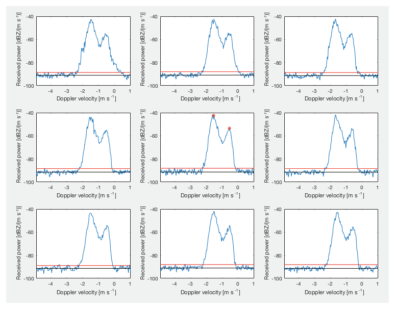
Figure 1Example of graphical user interface for peak-marking by hand. For the Doppler spectrum in the center panel, two peaks (red stars) were marked by the user (HK). The surrounding panels display the spatially and temporally neighboring spectra. Data are as follows: KAZR spectra observed at TMP on 16 February 2014, 0.03–0.05 UTC, between 1.0 and 1.2 km height. The red line marks the maximum noise floor determined according to Hildebrand and Sekhon (1974), and the black line the mean of the noise.
3.1 PEAKO algorithm description
In this study, a supervised Doppler spectra peak-finding algorithm (in the following text referred to as PEAKO) was developed, which was trained via hand-marked Doppler peaks as input. The learning process was split into two phases, the training phase and the test phase. For that purpose, three data sets, each containing example input and the corresponding desired output, were created:
-
a first training data set, used to obtain an initial model;
-
a second training data set, about half as large as the first training data set, used to tune the model;
-
a testing data set, which is approximately the same size as the second training data set, used for model evaluation.
With the help of a graphical MATLAB interface, in which the currently to-be-marked Doppler spectrum and its surrounding neighbors (in time and height) are displayed in logarithmic space (see Fig. 1), pronounced Doppler spectrum peaks were hand-marked by an experienced user. Even though this approach is subjective, criteria such as peak width, dynamic range, i.e., the height above noise floor, skewness of the spectrum, and consistency of the feature (peak) in time–height were taken into account. The locations of these hand-marked peaks (in mean Doppler velocity (VD) units, m s−1), as well as their corresponding signal powers (dBZ), were then saved as data matrices.
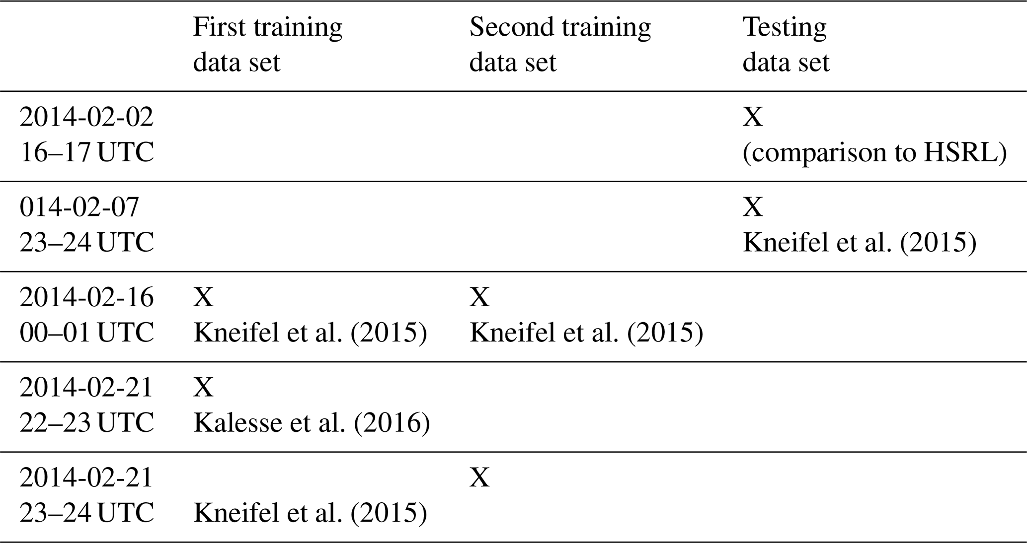
The training and test data sets were chosen as individual nonoverlapping time–height areas rather than randomly splitting all hand-marked spectra into training and test categories. For the training phase, data recorded on 21 February 2014, 22–23 UTC were utilized, a time period which was studied in greater detail before (Kalesse et al., 2016; Mason et al., 2018). Data from 16 February 2014, 00–01 UTC, which were in part investigated in a case study presented in Kneifel et al. (2015), were used in the training phase as well. The third case selected for the training data set, 21 February 2014, 23–24 UTC, was in part analyzed by Kneifel et al. (2015) as well. The test set is comprised of two 1 h cases, which were recorded on 2 February 2014, 16–17 UTC, and on 7 February 2014, 23–24 UTC. In the case of 2 February 2014, 16–17 UTC, the study area was set within the lowest liquid layer where independent HSRL measurements were used to check the performance of the PEAKO algorithm for liquid-peak detection. Unfortunately, the HSRL was fully attenuated by near-surface liquid layers during the other case studies. The chosen period on 7 February 2014 overlaps with another case investigated by Kneifel et al. (2015). Table 1 gives a summary of which measurement periods were used for which of the data sets.
Kneifel et al. (2015)Kneifel et al. (2015)Kneifel et al. (2015)Kalesse et al. (2016)Kneifel et al. (2015)Table 1Overview of the measurement periods used in each of the three data sets (first training data set, second training data set, testing data set) containing hand-marked peaks. Published studies of the selected periods, to which results can be compared, are noted as well.
The PEAKO algorithm includes a set of three subsequently described adjustable parameters (smoothing span, prominence threshold, minimum peak width at half-height), which are varied to obtain the set of parameters which yields the best agreement of hand-marked and machine-marked peaks. The search for the best parameter combination is done via a search through a finite set of values in the three-dimensional search space.
As a first step, the raw spectrum at the current time and height is replaced by an average spectrum obtained by averaging 27 spectra, 9 in time and 3 in height centered on the current one. For the given KAZR time–height resolution of 2 s (time) and 30 m (range), this translates to averaging of 18 s in the temporal dimension and 90 m in the spatial dimension. With hydrometeor populations usually appearing in distinct layers, which are persistent over a certain period of time, more neighbors in time than height are used for averaging. Figure 9a in Buehl et al. (2016) shows minimum liquid layer depths on the order of 50 to 100 m equivalent to two to three range gates assuming 30 m vertical range gate spacing, which motivated our choice of 90 m. The averaged spectrum is then further smoothed using local polynomial regression. The smoothing method applied, locally estimated scatterplot smoothing (loess), performs weighted linear least-square fitting on consecutive subsets of adjacent data points with a second-degree polynomial model. The span for smoothing is the fraction of the total number of data points (here Doppler bins) of one Doppler velocity spectrum to be used for each local fit. Loess was chosen empirically after testing different methods because it showed the best ability to capture peaks while filtering out noise. The span is varied in a range between 3.5 % and 13 %, regularly spaced with a distance of 0.5 %.
In the next step, local maxima are identified in the averaged and smoothed spectrum. Only peaks with powers above the raw spectrum's maximum noise are considered. Finally, peaks with prominences below the prominence threshold and widths smaller than the minimum peak width are excluded.
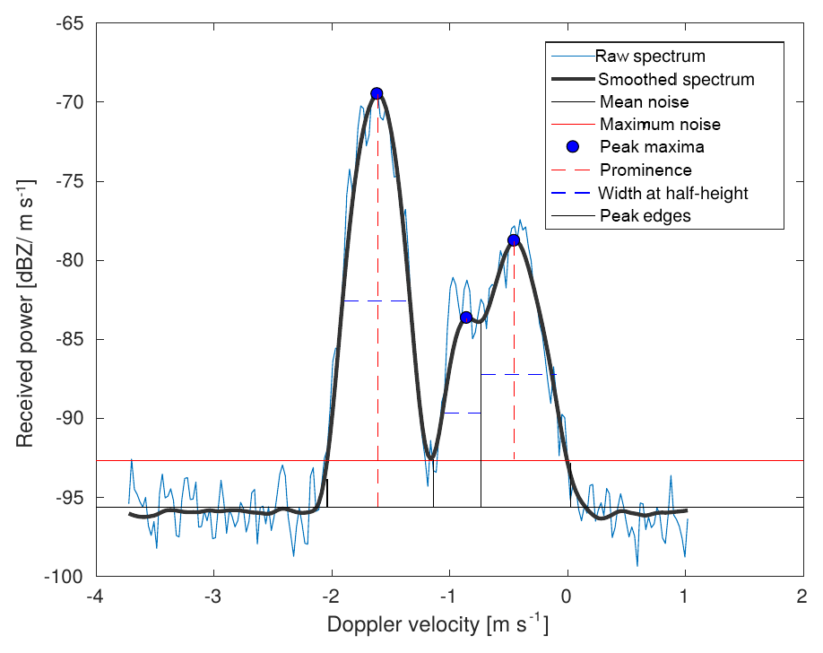
Figure 2Example spectrum (blue line) with multiple merged peaks, recorded on 21 February 2014, 22.7 UTC, at 2.44 km altitude. The smoothed spectrum (average of neighbor spectra in time and height domain, smoothed using a span of 8.5 %) is shown as well (bold black line). For each of the three peaks marked in this spectrum (blue dots), the prominences (red dashed lines) and widths at half-height (blue dashed lines) as well as the edges (vertical black lines) of the peaks are marked. The red horizontal line marks the maximum value of the power in the raw (blue) spectrum among those Doppler spectral bins identified as noise by Hildebrand and Sekhon (1974). The black horizontal line is drawn at the mean power of the Doppler bins containing only noise.
The prominence threshold is a measure of how much a peak stands out relative to the other peaks in the considered Doppler spectrum. The prominence of a peak is the power difference (dynamic range) of the peak's maximum and the signal's minimum between the considered peak and the nearest higher peak. Concerning the highest peak of the Doppler spectrum, the prominence is the power difference between the peak maximum and the mean of the spectral noise determined by Hildebrand and Sekhon (1974). This parameter is varied between 0 and 2 dBZ m−1 s−1 in the training phase of PEAKO. Figure 2 illustrates the definition of the peak prominence: a spectrum with three merged peaks is shown and their prominences are drawn as red vertical lines. In the case of the rightmost peak ( m s−1), the prominence is defined as the power difference between the peak's maximum and the minimum between this peak and the nearest higher peak. This minimum is located approximately at the leftmost peak's right edge (marked with a solid black vertical line at around −1.1 m s−1). For the peak with the lowest power at m s−1, the prominence of 0.25 dBZ m s−1 is barely visible because it is defined as only the distance between this peak's maximum and the minimum to the closest higher peak, which is the peak with the lowest absolute VD.
The third adjustable parameter is the minimum peak width at half-height. The range of values in which it is varied (4.2 to 8.4 Doppler velocity bins, spaced with a distance of 1.05) was determined from a low-turbulence cloud region only consisting of liquid droplets (21 February 2014, 22.53–22.59 UTC 2.9–3.1 km). Doppler spectra peaks in low-turbulent liquid cloud droplet layers are very narrow and thus suited to determine the minimum width of a peak considered physically meaningful. At the given KAZR resolution, these peaks were found to be between 4.2 and 8.4 VD bins wide corresponding to about 10–20 cm s−1.
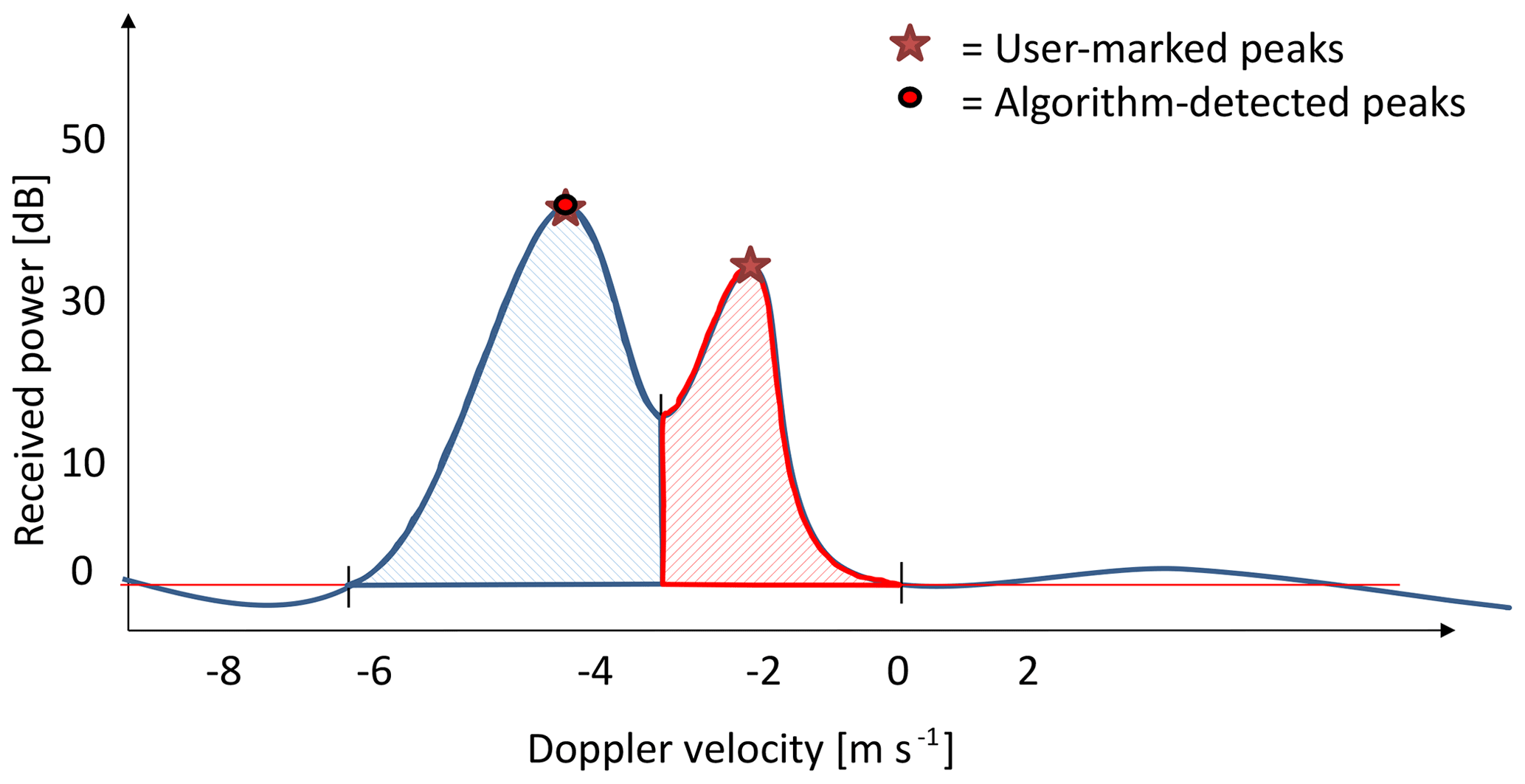
Figure 3Schematic to visualize how the similarity measure to compare user-marked and algorithm-found peaks in Doppler spectra: areas of matching peaks are summed up (blue hatched area), and the areas of mismatched peaks (red hatched) are subtracted.
To determine the optimal parameter combination, a similarity measure is defined, based on the maximum overlapping area of detected peaks as illustrated in Fig. 3: for a certain set of smoothing span, minimum peak width, and prominence threshold, the algorithm will detect certain peaks in a Doppler spectrum (shown as red dots surrounded by blue circles in Fig. 3). For these peaks, as well as for the peaks marked by a user in the same Doppler spectrum (red stars in Fig. 3), the edges (marked with vertical lines) are determined, which are defined as follows. The edge is either the first Doppler bin where the spectrum power is smaller than the maximum noise floor or, in the case of a merged peak, the minimum (saddle point) between the merged peaks. In the next step, the overlapping area for each pair of hand-marked and machine-found peaks is identified. In the case of multiple peaks in one spectrum, the sum of all overlapping areas is determined. Nonoverlapping regions caused by either a mismatch in the number of hand-marked and machine-found peaks or a different location (in x direction, i.e., in Doppler velocity) of the pair of peaks are penalized by subtracting the nonoverlapping area (red hatched area in Fig. 3) of the mismatched peaks from the similarity area measure. The optimum parameter combination is the triplet of span, prominence threshold, and minimum peak width for which the similarity has its maximum value.
3.2 Description of other radar Doppler spectra peak-finding algorithms
Three other radar Doppler velocity spectrum peak-finding algorithms were compared to PEAKO and will be briefly explained in the following.
The algorithm described in Shupe et al. (2004) (from now on referred to as “Shupe_04”) uses peak-finding criteria optimized to one relatively short (30 min) mixed-phase cloud case study period. In short, the power of the primary (strongest) peak must be at least 4 standard deviations of the noise above the mean spectral noise level. In addition, one or more secondary peaks are identified as maxima being at least 2.5 standard deviations of the noise greater than the mean spectral noise level. Both primary and secondary peaks must have a width of at least 0.448 m s−1. Merged peaks are identified as separate spectral modes if the saddle point between the two maxima is lower than 65 % of the lowest of the two peaks from the noise level.
The MicroARSCL data product (Kollias et al., 2007; Luke et al., 2008) decomposes noise-floor-subtracted and three-bin-boxcar-filtered radar Doppler spectra into a primary peak (defined as the peak containing the bin with maximum spectral power density), dominating the total reflectivity and containing up to two sub-peaks, and a possible secondary peak. Fixed thresholds, i.e., minimum primary or secondary peak width (Pwmin), minimum sub-peak height (Phmin), minimum sub-peak separation (Psmin), and minimum primary–secondary peak edge separation (Pnmin), are applied to extract a suite of variables from the Doppler spectra. Pwmin is set to five Doppler velocity bins (0.12 m s−1), Psmin to three Doppler velocity bins (0.07 m s−1), Pnmin to one Doppler velocity bin (0.0237 m s−1), and Phmin to 1 dBZ m−1 s−1. For the comparative study, a third technique, a polynomial fitting algorithm as described in Kollias et al. (1999, 2003), was also applied to the radar Doppler spectra that are analyzed in this study. This routine first extracts the parts of the spectrum above the maximum noise floor (the noise threshold determined by Hildebrand and Sekhon, 1974) and extends the edges of the found peaks down to the mean noise floor. In a next step, each continuous sample of data above the noise floor is identified as a sub-spectrum. Sub-spectra that are classified as being too narrow (with velocity ranges of the peak smaller than 0.2 m s−1) are excluded. For each of the remaining sub-spectra, polynomial fitting of the 12th order is applied. The first and second derivatives are taken to identify minima and maxima. Peaks are defined as sequences of minimum–maximum–minimum. Peaks having a velocity range smaller than 0.2 m s−1 are ignored, as well as peaks with an amplitude smaller than 2 dB, with amplitude being defined as the difference in reflectivity between consecutive minimum and maximum.
The following section will be structured as follows: in Sect. 4.1, the best parameter values obtained during the training phase of the PEAKO algorithm are summarized. The peaks detected by one of these best parameter combinations are compared to peaks found by the Shupe_04, MicroARSCL, and Polyfit12 algorithms in a case study. It should be noted that PEAKO was trained with a subset of data from the same distribution as this firstly presented case study. This means that PEAKO has somewhat of an advantage over the other three algorithms when comparing to the training data set. Section 4.2 summarizes the testing phase and presents a comparative independent study case, in which PEAKO-found peaks are again compared to peaks detected by the three other algorithms and validated against HSRL retrievals of liquid water droplets. More case studies are presented in the Appendices.
4.1 Training phase of the PEAKO algorithm
The training phase was split into two steps: Initially, peaks marked manually in 1340 Doppler spectra were used for training the PEAKO algorithm and obtaining an initial model via a coarse parameter search. This initial training resulted in six equally well-performing combinations of span, prominence threshold, and width, which all yield the same value of the similarity measure. A more finely resolved search for the three parameters was then performed, using 775 Doppler spectra with user-marked peaks. This second, refined training again resulted in several combinations of minimum peak prominence, minimum peak width, and smoothing span yielding the same similarity. Table 2 gives an overview of the possible ranges found for the three PEAKO parameters after the initial training and the more finely resolved parameter search. The span for loess became slightly larger (increased by 0.5 %–1 % in absolute terms) and converged to one single possible value (8.5 %). The minimum peak prominence decreased by one-third, i.e., from 0.15 to 0.1 dBZ m−1 s−1. This prominence threshold is very low compared to values used by other peak-finding techniques. However, in other approaches, spectra are usually not smoothed and neighbor-averaged. Maxima prominent enough in time and height to be still visible after averaging and smoothing are most probably physical, justifying the low prominence threshold. The possible values for the minimum peak width did not change significantly between the initial and the more refined model and ranges between 0.09 and 0.15 m s−1 (i.e., VD range, from 4 to 6.25 VD bins for the given KAZR Doppler spectra resolution). Doppler spectrum peaks detected by PEAKO configured in one of these combinations (span = 8.5 %; prominence threshold = 0.1 dBZ m−1 s−1; minimum peak width = 4 m s−1) are compared to peaks found by other methods for a study case on 21 February 2014, 22.54 to 22.77 UTC, at 2 to 6 km height. This parameter set containing the smallest possible minimum peak width was chosen because it is most stringent and thus best suited for the detection of narrow supercooled liquid water peaks. The selected period was discussed in detail in Kalesse et al. (2016).
Table 2Ranges of the parameters yielding the highest similarity measure after the initial and the finely tuned training using the first and second training data sets, respectively.
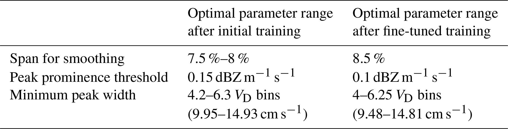
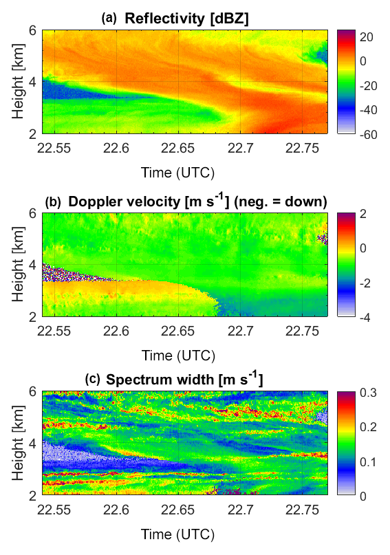
Figure 4Case study period from 21 February 2014, 22.54 to 22.77 UTC, at 2 to 6 km height. Panels (a), (b), and (c) show the radar reflectivity factor Ze, the mean Doppler velocity (MDV), and the Doppler spectrum width σ of the main peak in the Doppler spectrum.
Figure 4 shows the first three radar moments, i.e., the radar reflectivity factor Ze, the mean Doppler velocity (MDV), and the Doppler spectrum width σ for the first selected case study, which is set from 21 February 2014, 22.54 to 22.77 UTC, at 2 to 6 km height. This time period is characterized by the passage of a warm occlusion in Hyytiälä, Finland, shown by the continuously lowering frontal snow cloud base characterized by high Ze. A mid-level mixed-phase cloud was present before the front approached. It can be identified by its supercooled liquid water (SLW) layer near cloud top between approximately 2.9 and 3.2 km altitude. Before the snow cloud moves in (22.54 to 22.69 UTC), new ice is formed from this SLW layer and grows in size while sedimenting, leading to a slight increase in Ze, MDV (absolute value), and σ with decreasing altitude. As the frontal cloud moves in and snow begins to fall through the SLW layer, riming takes place along slanted fall streaks. A more in-depth analysis of the synoptic situation and the observed microphysical growth processes is given in Kalesse et al. (2016).

Figure 5Number of Doppler spectrum peaks detected by different algorithms for the selected case study on 21 February 2019 from 22.54 to 22.77 UTC at 2 to 6 km altitude. (a–d) Number of peaks found by the PEAKO algorithm for one of the “best parameter” combinations obtained in the training phase of the algorithm; number of peaks in MicroARSCL data product; number of peaks detected using the criteria of Shupe_04; number of peaks determined by Polyfit12.
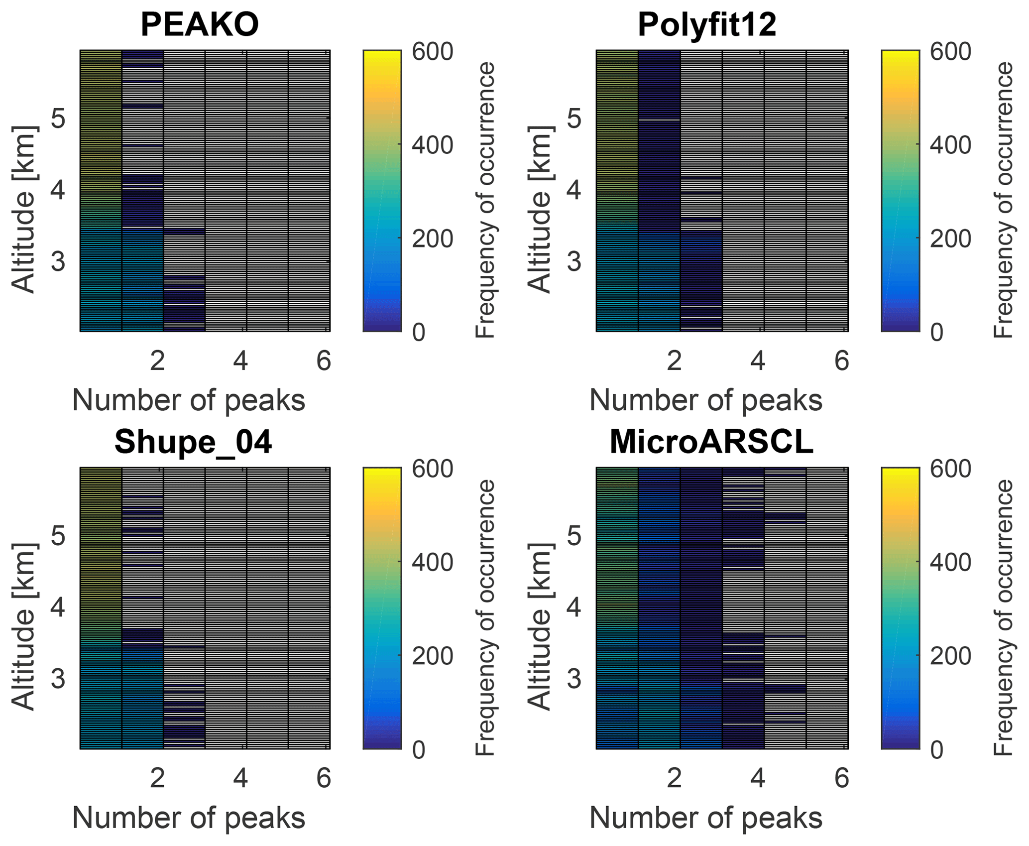
Figure 6Contoured frequency by altitude diagram (CFAD) for the frequency of occurrence of number of detected peaks from different algorithms for the case study period on 21 February 2014 from 22.54 to 22.77 UTC at 2 to 6 km altitude.
The number of detected peaks for this case study is shown in Fig. 5. All algorithms show a similar general picture with an increasing number of spectral peaks as the snow front moves in and snow starts falling through the SLW layer of the mid-level mixed-phase cloud. A closer examination however reveals some differences between the methods: the PEAKO and Shupe_04 algorithms have very similar results except for some areas in the snowfall region where PEAKO detects three peaks and Shupe_04 detects two peaks. MicroARSCL generally shows higher variability than the other algorithms; the small areas of higher peak number often coincide with increased spectrum width in Fig. 4. Polynomial fitting shows three peaks in the area where snow falls through the top of the SLW layer and is otherwise very similar to PEAKO and Shupe_04. The areas where the different algorithms show discrepancies are now examined in more detail.
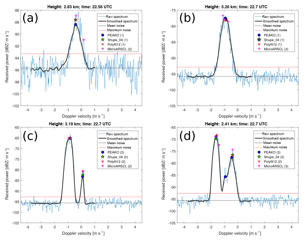
Figure 7Four exemplary Doppler spectra picked from the case study on 21 February 2014, 22.54 to 22.77 UTC, at 2 to 6 km altitude. The averaged and smoothed spectrum which is used as input to PEAKO is drawn in bold over the original spectrum. The peaks detected by the four algorithms are marked. The number of peaks found by each algorithm is noted in parentheses in each figure legend. Please note the different y scales.
For that purpose, contoured frequency by altitude diagrams (CFAD, Fig. 6) is created to compare the results of the algorithms in a different way. The CFAD shows the number of detected peaks (abscissa) at different heights (ordinate) as a colored frequency of occurrence for the total case study sample. For all four compared algorithms, it is most common that only one peak is detected. This is especially true for higher altitudes within the snow front (4 km and above). It is visible that the PEAKO algorithm and the results obtained using the Shupe_04 approach agree to a large extent. In the polynomial fitting approach, two or three peaks are detected more often, especially in the layer just above 3 km altitude, where several spectra are classified to contain three peaks. The MicroARSCL data product contains even more Doppler peaks, often three or more, over the complete altitude range.
In Fig. 7, four exemplary spectra from regions where the algorithms show discrepancies are shown along with the peaks detected by each of the four algorithms. The spectrum in Fig. 7a is recorded in 2.83 km height at 22.56 UTC, below the SLW and before the snow front moves in. As discussed in Kalesse et al. (2016), ice particles which are nucleated in the SLW layer of the mid-level cloud and growth through water vapor deposition lead to this Gaussian-shaped monomodal Doppler peak. The spectrum is relatively broad (as can also be seen from Fig. 4) and noisy, pointing to turbulence. MicroARSCL is sensitive to small-scale noise of the original spectrum, which the other algorithms are not sensitive to, and thus overestimates the number of spectral peaks. Figure 7b shows a spectrum from later on, at 22.7 UTC, in the upper part of the frontal snow cloud at 5.26 km height. In this time–height region, PEAKO, Shupe_04, and Polyfit12 detect the Gaussian-shaped snow peak, but MicroARSCL is again sensitive to small-scale fluctuations in the Doppler spectra and finds three peaks. The example in Fig. 7c is taken from 3.2 km altitude at 22.7 UTC where snow from the frontal cloud starts to fall through the SLW. All four algorithms are able to detect the very narrow noise-floor-separated peak produced by the supercooled liquid droplets with VD near 0 m s−1. Figure 7d shows a spectrum recorded at the same time but below the SLW layer at 2.41 km height, where freshly generated ice ( m s−1), unrimed snow ( m s−1), and rimed snow ( m s−1) are present. These hydrometeor populations do not have sufficient differences in terminal fall velocities and thus produce a spectrum with merged peaks. For this example, Shupe_04 and Polyfit12 detect the two main maxima (freshly generated ice and rimed snow), whereas MicroARSCL and PEAKO find three peaks. However, closer examination of the example spectrum shows that the two algorithms each detect an additional peak in different locations: MicroARSCL finds a sub-peak in the faster falling hydrometeor population (the Gaussian peak of the rimed snow) while PEAKO detects a sub-peak in the slower-falling mode, which exhibits a strong skewness. This sub-peak is most likely caused by snow from the upper layers, which remained unrimed as discussed in Kalesse et al. (2016).
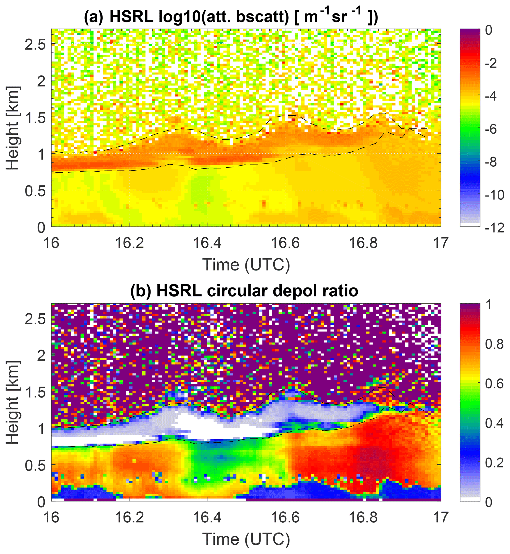
Figure 8HSRL measurements from the case study period from 2 February 2014 from 16 to 17 UTC at 0 to 3 km height. Panel (a) shows the attenuated backscatter cross section and panel (b) the circular depolarization ratio. The black dashed line marks the boundary of the supercooled liquid layer, indicated by high backscatter and low depolarization ratio.
The results of the PEAKO comparison to the other three peak-finding approaches for the other two training data sets, i.e., for 16 February 2014, 0.67 to 0.92 UTC, and for 21 February 2014, 23.01 to 23.25 UTC, are shown in Appendices A and B. Time–height plots of peak number are shown in Figs. A2 and B2; CFAD diagrams can be found in Figs. A3 and B3. Both of these time periods were also analyzed by Kneifel et al. (2015) in depth, so it was possible to compare the microphysical signatures reported in this study to the Doppler peaks detected by the four algorithms. For 16 February 2014, 0.67 to 0.92 UTC, Kneifel et al. (2015) reported high values of microwave-radiometer-derived liquid water path of 100 to 500 g m−2 and clear signatures of large aggregates in the dual-wavelength ratios of Ka-band to W-band reflectivities below 2 km as well as in the reflectivity fall streak feature at 0.85 UTC, which were also seen in the X–Ka dual-wavelength ratios around 0.85 UTC. The general structure of the layers of Doppler peak number detected by PEAKO, Shupe_04, and Polyfit12 again agree to a large extent, whereas MicroARSCL detects a higher number of peaks in both cases (Figs. A2 and B2). The fall streak feature which exhibits particle size sorting was better detected by PEAKO and MicroARSCL than by the other two algorithms. The increase in number of peaks at 0.67 to 0.75 UTC can be explained by the presence of large needle aggregates of sometimes more compact and sometimes very open structure as explained in Kneifel et al. (2015), which lead to the interesting multimodal Doppler spectrum with up to four peaks as shown in Fig. B4d. Ground-based in situ observations show that during 0.75–0.85 UTC aggregates and rimed particles with enhanced terminal velocities were present and that the number of large aggregates was further found to decrease while number of increasingly rimed aggregates further increased until 1 UTC. Radio-sounding observations on 15 February 2014 at 23.2 UTC show a thin layer at 0.8–0.9 km altitude, which is subsaturated with respect to ice and liquid and which might explain the decrease to one found Doppler peak at this altitude. For 21 February 2014, 23.01 to 23.25 UTC, Kneifel et al. (2015) report the transition from a low concentration of strongly rimed particles (lump graupel) to aggregate snowfall with large snowfall rates and increasing size and number of the aggregates. The fast transition of the snowfall from rimed particles to aggregates results in the bimodal Doppler spectra (with two found peaks) at 23 to 23.05 UTC and monomodal spectra afterwards. For this case study, PEAKO and Shupe_04 and Polyfit12 agree well with the situation described in Kneifel et al. (2015) while MicroARSCL overestimates the number of peaks, especially in the turbulent boundary layer and near 4 km altitude.
4.2 Testing phase of the algorithm
Using the tuned parameter pairs obtained in the training phase, the PEAKO algorithm is again compared to the other three algorithms, as well as to data measured by an independent instrument, the HSRL. For this purpose, a case of a frontal passage associated with snow on 2 February 2014, 16:00 to 17:00 UTC, was analyzed. During this time, a liquid-topped mixed-phase cloud with cloud top temperature of ( ∘C) and cloud top height of 2.6 km was present (Fig. 9). A deeper precipitating cloud system with cloud top around 8 km (cloud top temperature of −40 ∘C) was approaching the TMP site at about 16.27 UTC. The surface temperature was −5 ∘C. During the first half of the hour-long case study, the HSRL detected an embedded layer of SLW in the mid-level cloud, characterized by high backscatter coefficient values and low depolarization ratio values (Luke et al., 2010) in Fig. 8. The SLW layer is located between 0.8 and 1 km height and is slightly lifted as the front is moving in. Its base and top are traced with dashed lines in Fig. 8. After 16.8 UTC, the microwave-radiometer-derived liquid water path (LWP) decreases from around 300 g m2 to approximately 60 g m2 and the lidar does not detect the cloud base anymore due to the scarcity in small liquid droplets to which the lidar is sensitive and due to the strong snowfall. The strong decrease in LWP again points to riming. Analysis of the ground-based in situ particle imaging package (PIP) data shows a variety of different precipitating particles during that 1 h time period (Annakaisa von Lerber, personal communication, 2018): around 16 UTC, oblate particles, possibly needles, and some small needle aggregates are present. When Ze decreases around 16.3–16.55 UTC (Fig. 9), no large particles are present at all, just very small ones, maybe single pristine crystals (the resolution of PIP is not good enough to distinguish). At 16.55–16.8 UTC when Ze increases strongly and LWP decreases significantly, the PIP observes a clear change to round, dense, fast-falling particles, indicative of small graupel. Finally, from 16.8 UTC onward, particle sizes at the ground increase and there are more (quite dense) aggregates, resulting in Ze of up to 10 dBZ.
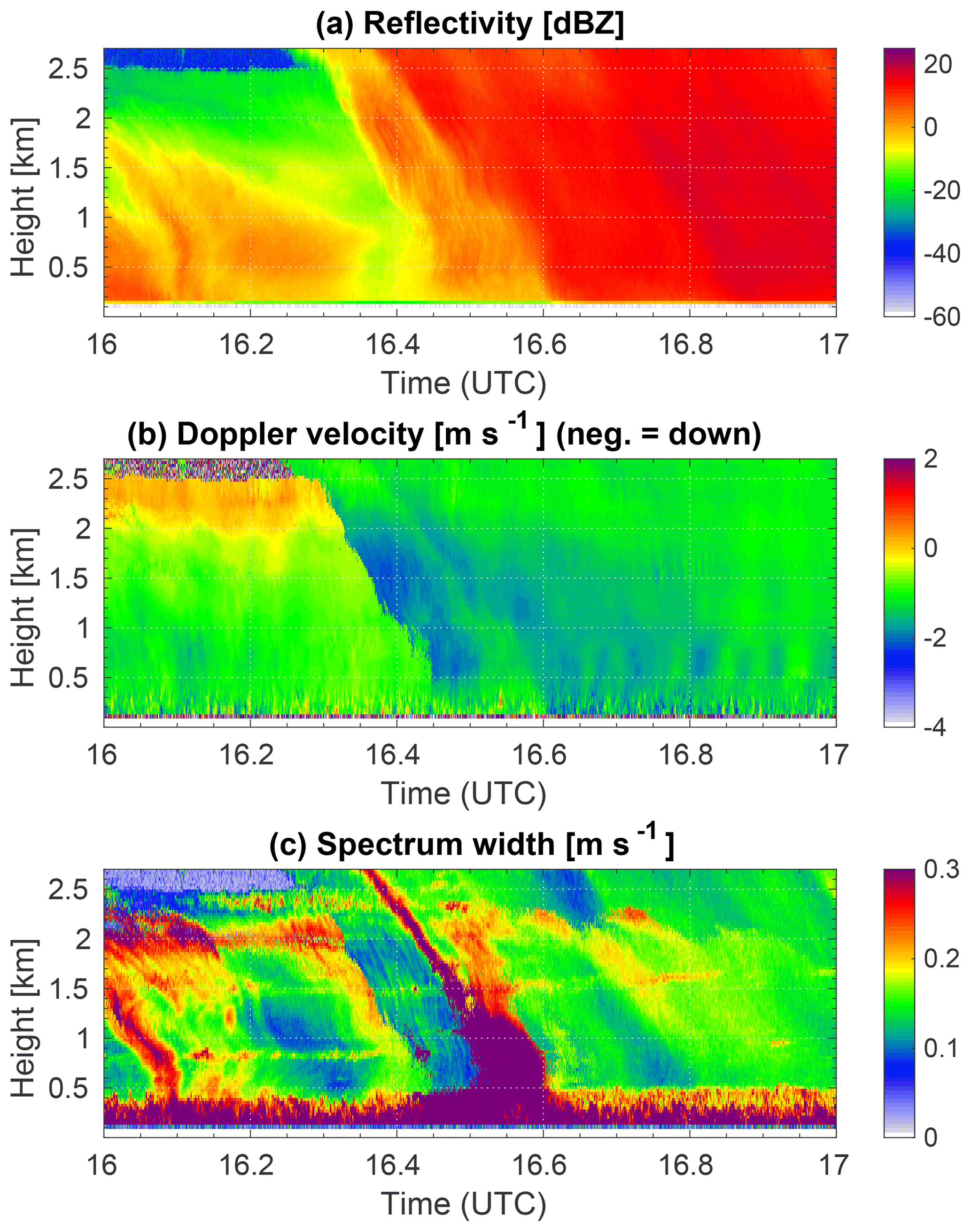
Figure 9 shows the first three radar moments (Ze, MDV, and σ) of the main peak for the selected case study. The supercooled liquid layer at the top of the mid-level cloud extends from about 2.1 to 2.4 km and is characterized by MDV of near 0 m s−1. Snow fall rate is at first low and increases at about 16.6 UTC (surface meteorological observations, not shown). Pronounced fall streaks can be seen coinciding with large values of spectrum width, indicating the presence of several hydrometeor populations, producing Doppler spectra with broad merged peaks.
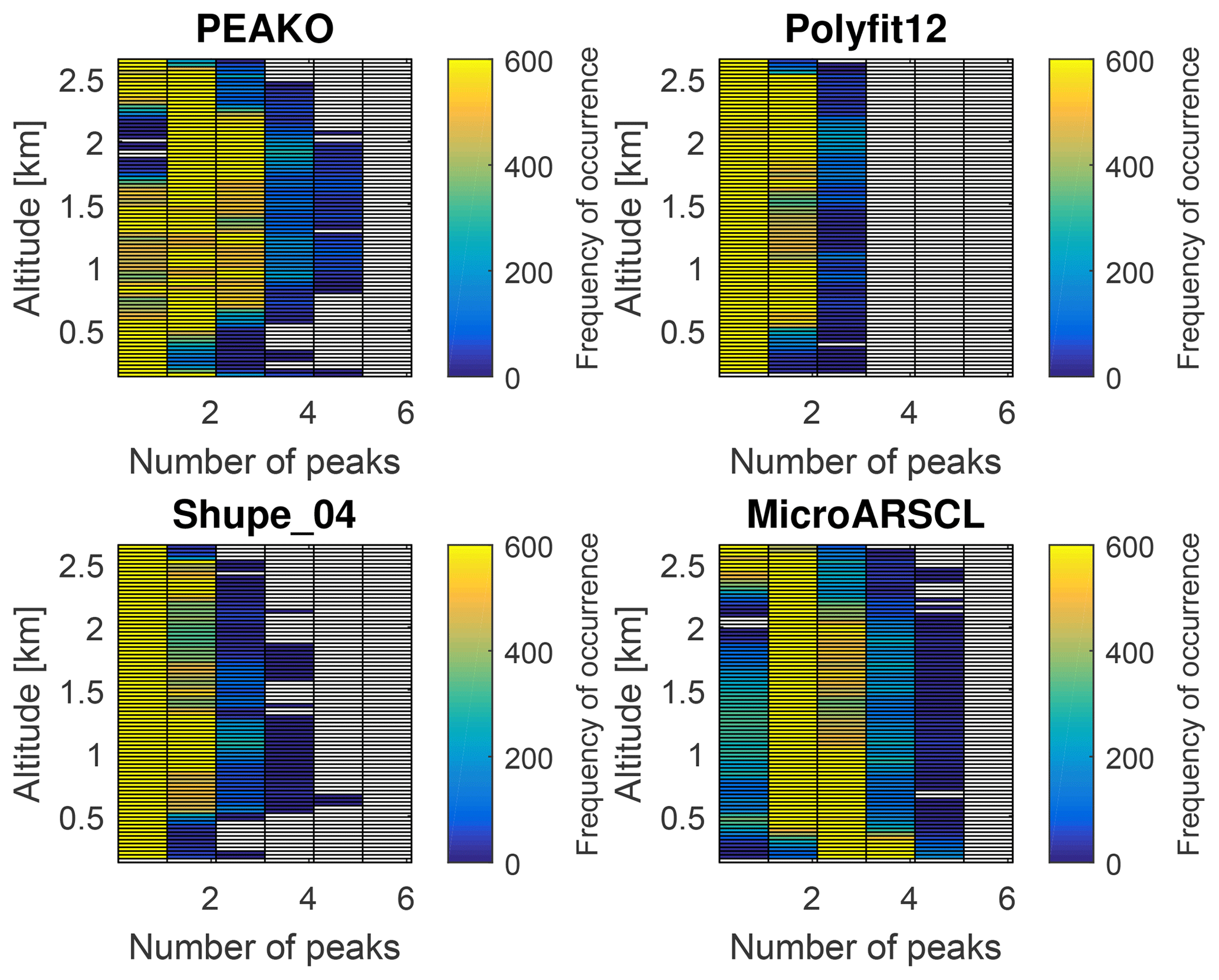
Figure 11Like Fig. 6 but for the case study period on 2 February 2014, 16:00 to 17:00 UTC, at 0 to 2.7 km altitude.
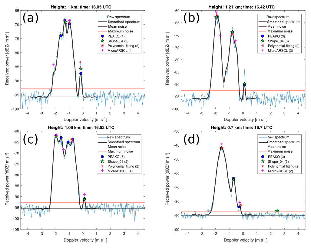
Figure 12Four exemplary Doppler spectra picked from the case study on 2 February 2014, 16:00 to 17:00 UTC, at 0 to 2.5 km altitude. The averaged and smoothed spectrum which is used as input to PEAKO is drawn in bold over the original spectrum. The peaks detected by the four algorithms are marked. The number of peaks found by each algorithm is noted in parentheses in each figure legend. Mean and maximum noise floors are presented by black and red horizontal lines, respectively. Please note that the scale of the y axis is different in each plot.
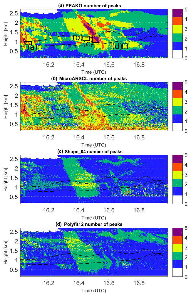
Figure 10 reveals that the number of peaks detected by the four algorithms differs significantly for this case study. Shupe_04 and Polyfit12 again agree to large extents, although Shupe_04 does mostly only detect one peak at 2–2.5 km height before 16.3 UTC and after 16.5 UTC where all other algorithms mostly detect two peaks. MicroARSCL generally detects a larger number of peaks in the Doppler spectra; PEAKO is in this case more similar to MicroARSCL than to the other two algorithms and often detects three to four and sometimes even five peaks along certain fall streaks. However, due to the smoothing performed within PEAKO, the detected features are less noisy and more consistent in time and height than for MicroARSCL.
Figure 11 shows CFAD diagrams for each of the four algorithms for the case study on 2 February 2014, 16 to 17 UTC. These graphs confirm that Polyfit12 and Shupe_04 estimate the number of peaks more conservatively than PEAKO and MicroARSCL. It is obvious that MicroARSCL often detects three or four peaks in the lowermost radar height bins, which can probably be attributed to turbulence. The HSRL-detected SLW layer (varying between 0.7 and 1.5 km height) is most obvious in the Shupe_04 and PEAKO CFAD plot; the number of spectra which are assigned two or three peaks is noticeably higher in this altitude range.
A closer look at the Doppler spectra substantiates the occurrence of riming during the selected study period: Fig. 12 shows four exemplary Doppler spectra from the case study on 2 February 2014, 16 to 17 UTC. Only PEAKO is able to detect a narrow peak near 0 m s−1 in all four example spectra. While these peaks can be attributed to SLW in Fig. 12a, b, and c, it is more likely that this small sub-peak in Fig. 12d is caused by small ice particles nucleated in the SLW layer situated slightly above because the HSRL does not detect liquid at 0.7 km altitude around 16.7 UTC. In addition to the peak near 0 m s−1, all shown spectra are characterized by broad merged snow peaks pointing to snow particles of different size, shape, and density falling at different terminal velocities. In Fig. 12a, the three merged modes of snow, as well as the SLW peak, are detected by PEAKO and MicroARSCL, while Shupe_04 and Polyfit12 both only detect one maximum.
The spectrum shown in Fig. 12b is near the top of the SLW layer detected by the HSRL. The narrow liquid peak with fall velocity near 0 m s−1 is only detected by PEAKO and Shupe_04. Both algorithms find two more snow peaks with larger fall velocity. These two peaks are also detected by Polyfit12. MicroARSCL detects three peaks as well; however it is not able to detect the liquid peak. Figure 12c shows a spectrum which was chosen in an area where PEAKO finds five peaks. Again, one of them is a SLW peak within the SLW layer detected by the HSRL (Fig. 10). This peak is also detected by MicroARSCL and Shupe_04 but not Polyfit12. The four other peaks found by PEAKO are merged snow peaks with different fall velocities which hint to various degrees of riming that the other algorithms have difficulties detecting. In Fig. 12d, the number of peaks detected by the four algorithms differs significantly: the peak with the highest reflectivity at around −1.5 m s−1 fall velocity is found by all algorithms. PEAKO detects two sub-peaks, which are each identified by at least one other algorithm as well. However, none of the other methods finds both other ice sub-peaks.
In Appendices A–C, three more case studies from the training and test phase are presented. Results of comparison of PEAKO to the other peak-finding algorithms are similar to the cases presented here. Appendix D contains a sensitivity study on the effect of different smoothing schemes and spatiotemporal averaging scales.
5.1 Summary of findings and outlook
The presented study focuses on the description of a new supervised cloud radar Doppler velocity spectrum peak-finding algorithm (PEAKO). Its performance was compared to different existing Doppler spectrum peak-finding algorithms. It was found that the PEAKO algorithm generally agrees well with results from Shupe_04 and a polynomial fitting approach. PEAKO is however capable of detecting narrower merged peaks with a smaller power contribution than Shupe_04. The polynomial fitting approach has mostly results similar to Shupe_04 but is not very practical due to its long computation time. The MicroARSCL product was usually more sensitive to small perturbations in the radar Doppler spectrum and thus often detected a higher number of peaks than the other three algorithms and produces more “speckled” results. Some areas where peaks are overestimated by MicroARSCL are in highly turbulent regions with large spectrum width like the turbulent boundary layer while others seem more random and not consistent in time and height. Consistency in time and to a lesser extent height is a good indicator of the performance of a peak-finding algorithm because hydrometeor populations and cloud microphysical processes generally occur in layers (unless in highly turbulent regions). The number of found cloud radar Doppler velocity spectrum peaks within mixed-phase wintertime snow clouds in Finland was validated with independent ground-based in situ observations described in Kneifel et al. (2015) and, if available, HSRL observations.
The described approach only identifies underlying hydrometeor populations if the particle types differ sufficiently in their terminal fall velocities to produce individual Doppler spectrum peaks.
In upcoming projects, it is planned to test if the best three-parameter pairs of PEAKO found are applicable to other radar systems (like METEK MIRA 35 GHz radars or RPG 94 GHz FMCW radars) or to which extent further refinement is needed for different radar sampling parameters. Additionally, the effect of stronger cloud dynamics will be evaluated.
Determining the number of different hydrometeor populations in the same radar volume based on morphological features of the radar Doppler spectrum as presented in this comparative study is the first step towards cloud particle classifications. Having this easily adjustable cloud radar Doppler spectrum peak detection algorithm available will facilitate carrying out microphysical process studies, involving applications such as peak tracking.
All KAZR and HSRL data of the second ARM Mobile Facility (AMF2) at the University of Helsinki Research Station (SMEAR II), in Hyytiälä, Finland, used in this study are publicly accessible at the ARM data archive: https://adc.arm.gov/armlogin/login.jsp (last access: 27 November 2018). The High Spectral Resolution Lidar (HSRL) data from 2 February to 21 February 2014 were compiled by B. Ermold, E. Eloranta, H. Michelsen, J. Garcia, J. Goldsmith, and R. Bambha. The data set was last accessed on 27 November 2018 at https://doi.org/10.5439/1025200 (Ermold et al., 2014). The Atmospheric Radiation Measurement (ARM) user facility Ka-band ARM Zenith Radar general moment data (KAZRGE) from 2 to 21 February 2014 were compiled by A. Matthews, B. Isom, D. Nelson, I. Lindenmaier, J. Hardin, K. Johnson, and N. Bharadwaj. The data set was last accessed on 27 November 2018 at https://doi.org/10.5439/1025214 (Matthews et al., 2014a). The Ka-band ARM Zenith Radar Doppler spectra data (KAZRSPECCMASKGECOPOL) from 2 to 21 February 2014 were compiled by A. Matthews, B. Isom, D. Nelson, I. Lindenmaier, J. Hardin, K. Johnson, and N. Bharadwaj. The data set was last accessed on 27 November 2018 at https://doi.org/10.5439/1025218 (Matthews et al., 2014b).
The results of the PEAKO comparison to the other three peak-finding approaches for the training data set of 16 February 2014, 0.67 to 0.92 UTC, are shown in Appendix A. This time period is also analyzed by Kneifel et al. (2015) in depth, so it was possible to compare the microphysical signatures reported in this study to the Doppler peaks detected by the four algorithms. For 16 February 2014, 0.67 to 0.92 UTC, Kneifel et al. (2015) reported high values of microwave-radiometer-derived liquid water path of 100 to 500 g m−2 and clear signatures of large aggregates in the dual-wavelength ratios of Ka-band and W-band reflectivities below 2 km as well as in the reflectivity fall streak feature at 0.85 UTC that were also seen in the X–Ka dual-wavelength ratios around 0.85 UTC. The general structures of the layers of Doppler peak number detected by PEAKO, Shupe_04, and Polyfit12 again agree to a large extent, whereas MicroARSCL detects a higher number of peaks in both cases (Figs. A2 and B2). The fall streak feature which exhibits particle size sorting was better detected by PEAKO and MicroARSCL than by the other two algorithms. The increase in number of peaks at 0.67 to 0.75 UTC can be explained by the presence of large needle aggregates of sometimes more compact and sometimes very open structure as explained in Kneifel et al. (2015), which lead to the interesting multimodal Doppler spectrum with up to four peaks as shown in Fig. B4d. Ground-based in situ observations show that during 0.75–0.85 UTC aggregates and rimed particles with enhanced terminal velocities were present and that the number of large aggregates was further found to decrease while the number of increasingly rimed aggregates further increased until 1 UTC. Radio-sounding observations on 15 February 2014 at 23.2 UTC show a thin layer at 0.8–0.9 km altitude which is subsaturated with respect to ice and liquid and which might explain the decrease to one found Doppler peak at this altitude.
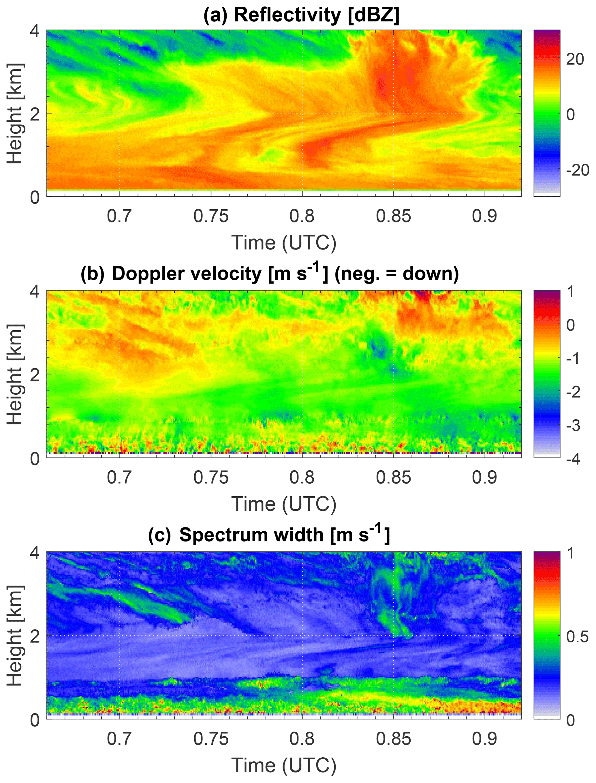
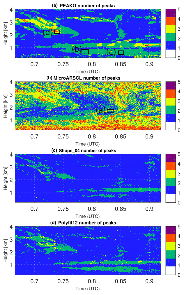
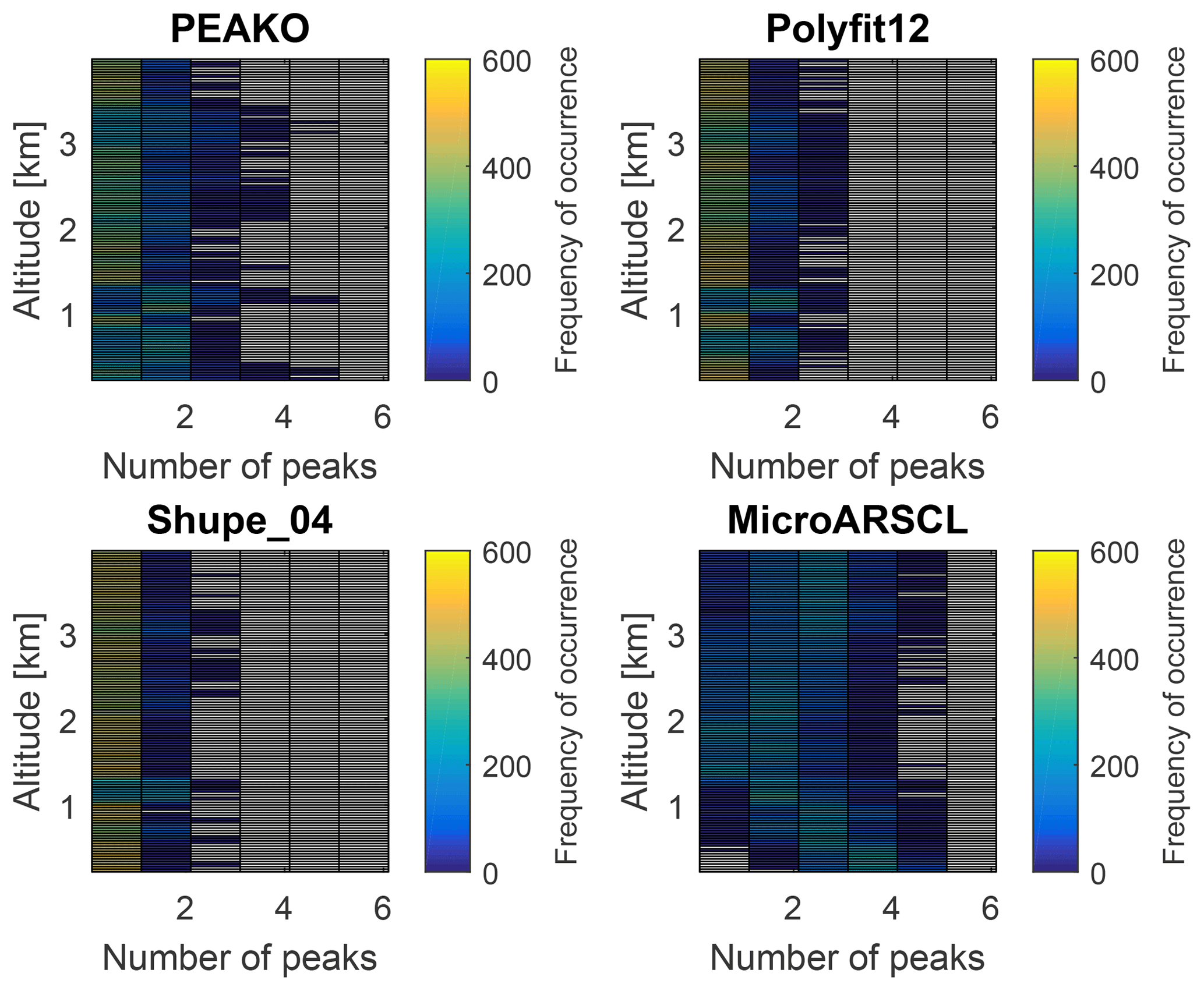
Figure A3Like Fig. 6 but for the case study period on 16 February 2014, 0.66–0.92 UTC, at 0–4 km altitude.
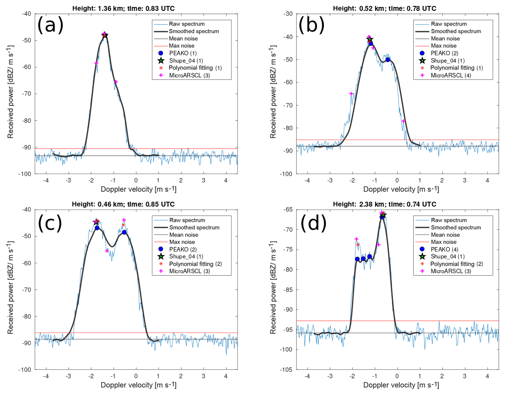
Figure A4Four example spectra selected from the case study on 16 February 2014, 0.63–0.92 UTC. Please note that the y axis scale is different for each of the spectrum plots.
The training data set of 21 February 2014, 23.01 to 23.25 UTC, which is also a case study of Kneifel et al. (2015), is described in Appendix B. For 23.01 to 23.25 UTC, Kneifel et al. (2015) report the transition from a low concentration of strongly rimed particles (lump graupel) to aggregate snowfall with large snowfall rates and increasing size and number of the aggregates. The fast transition of the snowfall from rimed particles to aggregates results in the bimodal Doppler spectra (with two found peaks) at 23 to 23.05 UTC and monomodal spectra afterwards. For this case study, PEAKO and Shupe_04 and Polyfit12 agree well with the situation described in Kneifel et al. (2015), while MicroARSCL overestimates the number of peaks, especially in the turbulent boundary layer and near 4 km altitude.
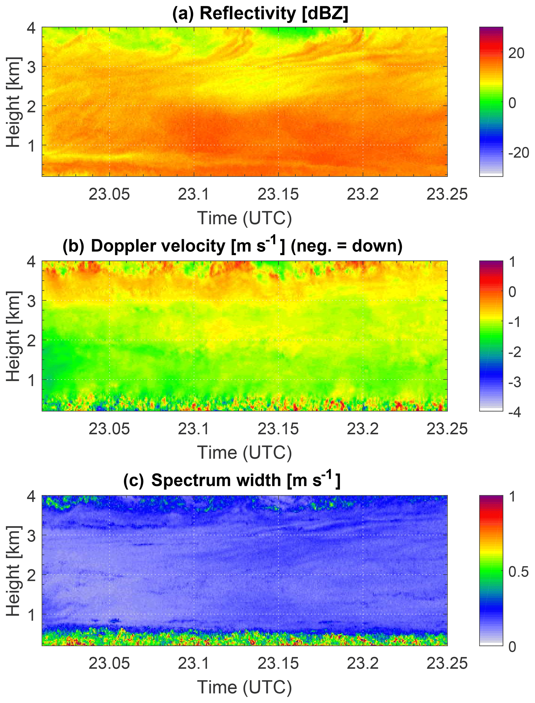
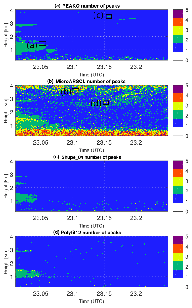
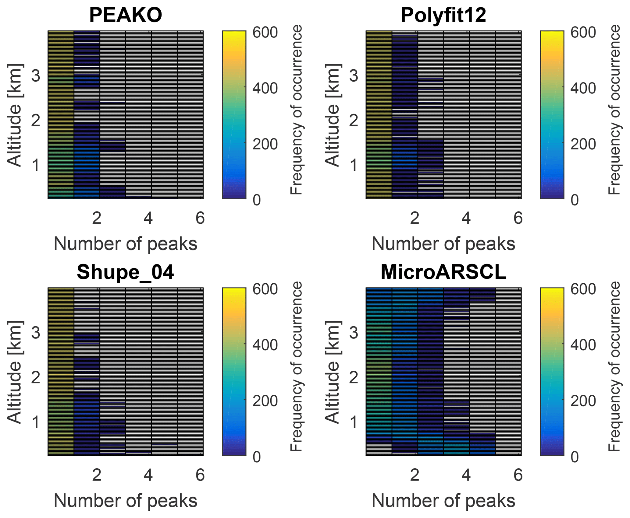
Figure B3Like Fig. 6 but for the case study period on 21 February 2014, 23.01–23.25 UTC, at 0.2–4 km altitude.
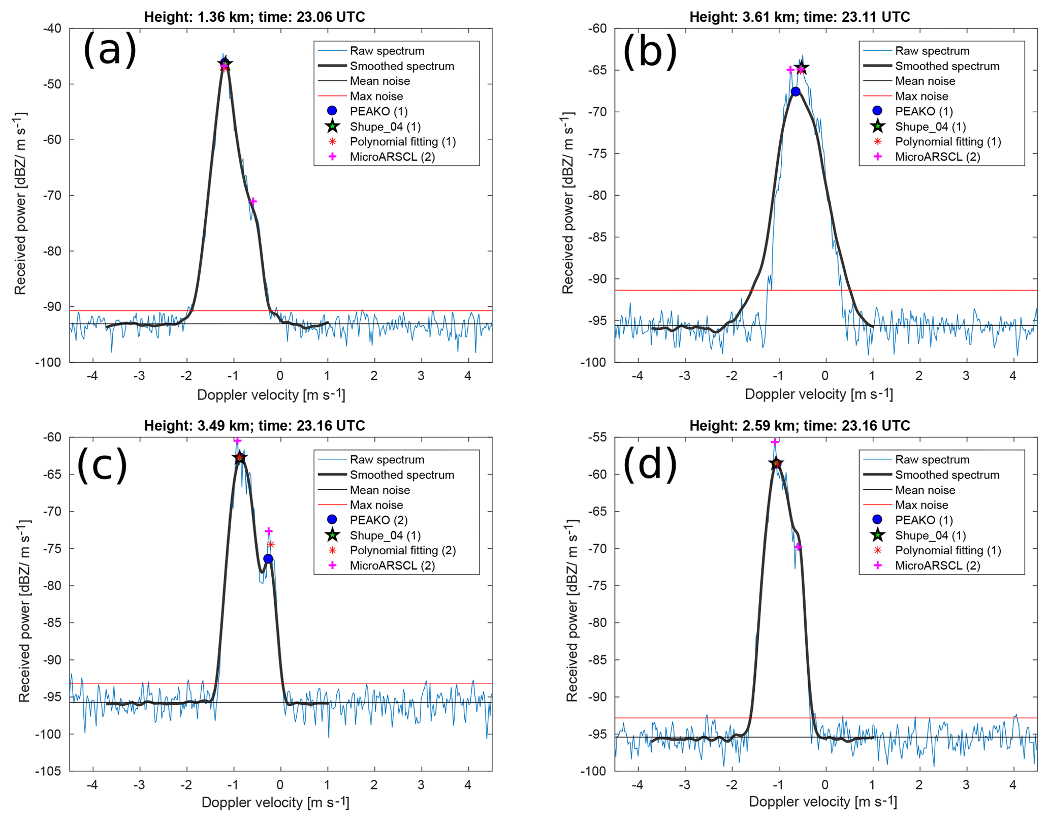
Figure B4Three example spectra selected from the case study on 21 February 2014, 23.01–23.25 UTC. Please note that the y axis scale is different for each of the spectrum plots.
The second test data set of 7 February 2014, 23.75 to 24 UTC, is characterized by dendritic ice particles (Kneifel et al., 2015) and a slanted fall streak feature extending from near 4 to 1 km from 23.75 to 23.9 UTC (Fig. C1) with bimodal Doppler spectra (Figs. C2 and C4). Ground-based in situ observations report mostly small, open-structured aggregates (which are later replaced by more compact spheroidal habits) as well as a small number of spherical probably rimed particles.
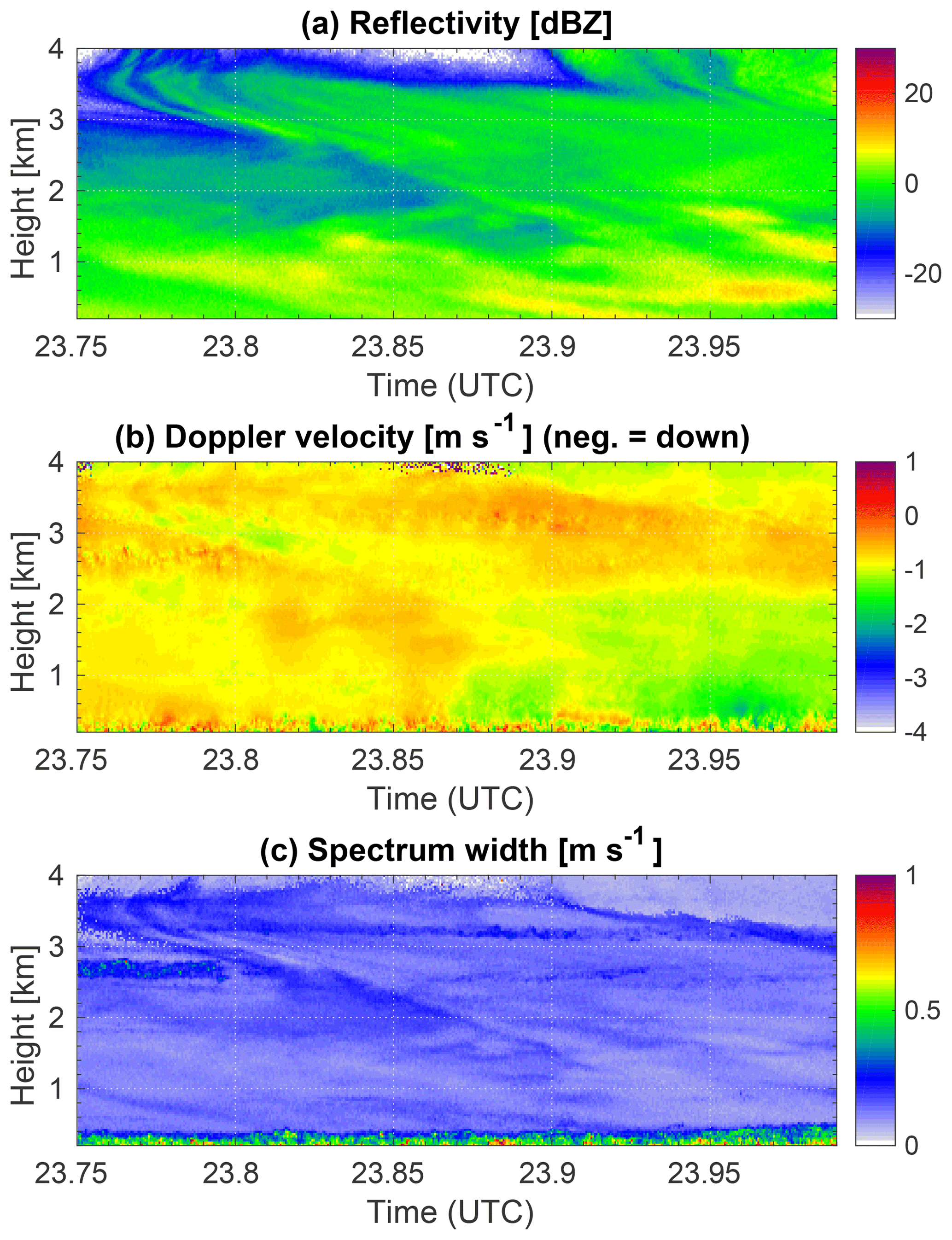
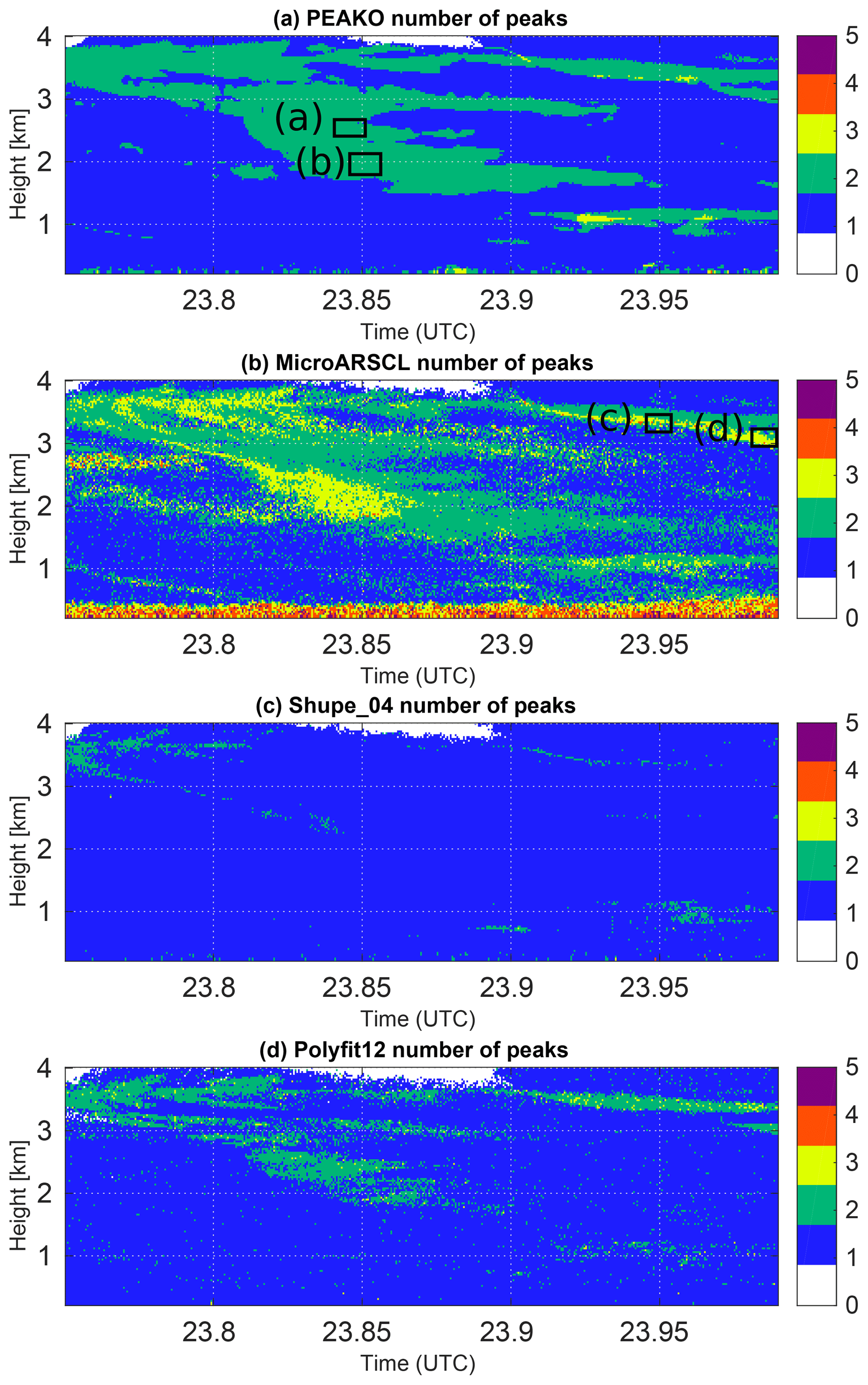
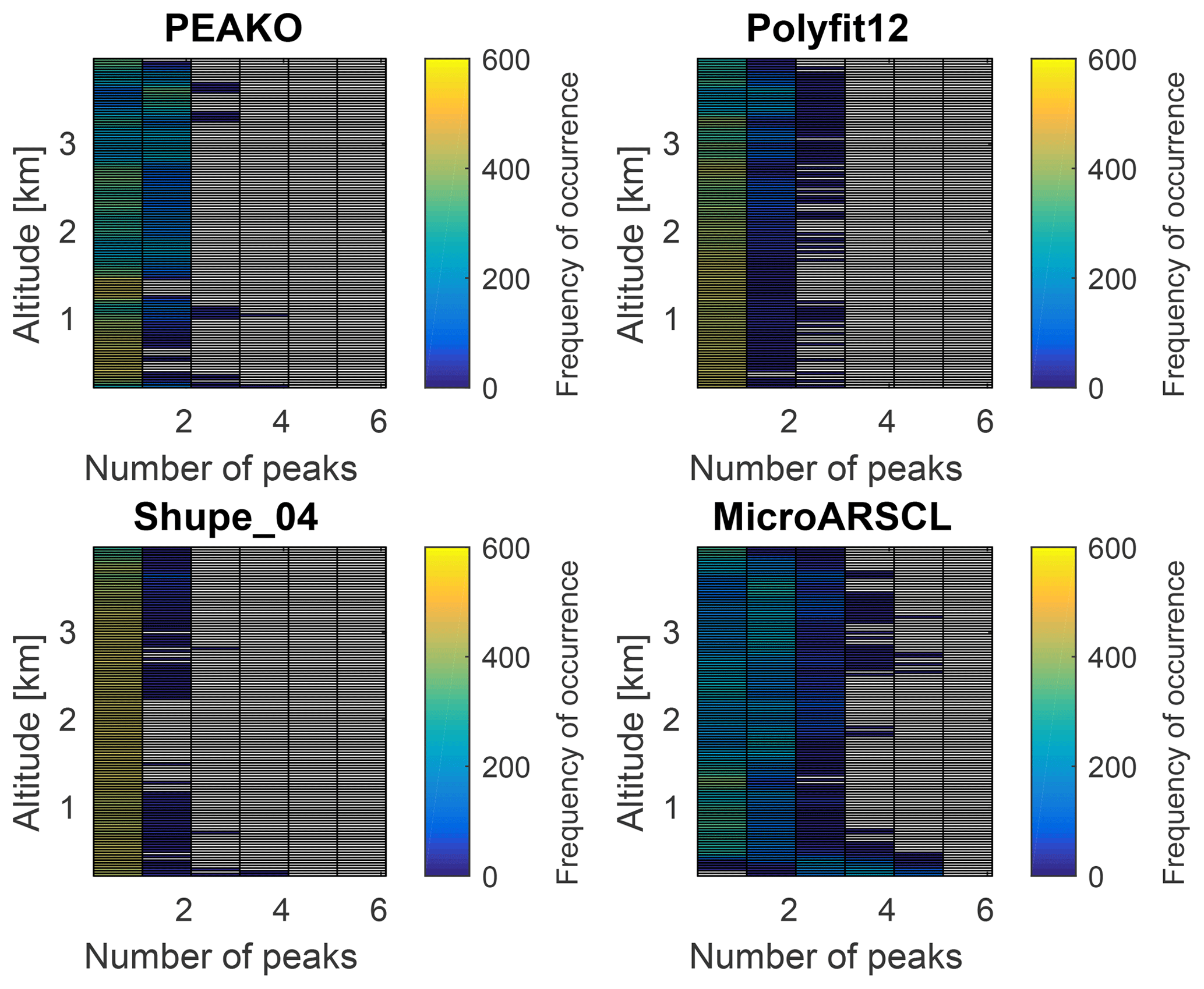
Figure C3Like Fig. 6 but for the case study period on 7 February 2014, 23.75–24 UTC, at 0.2–4 km altitude.
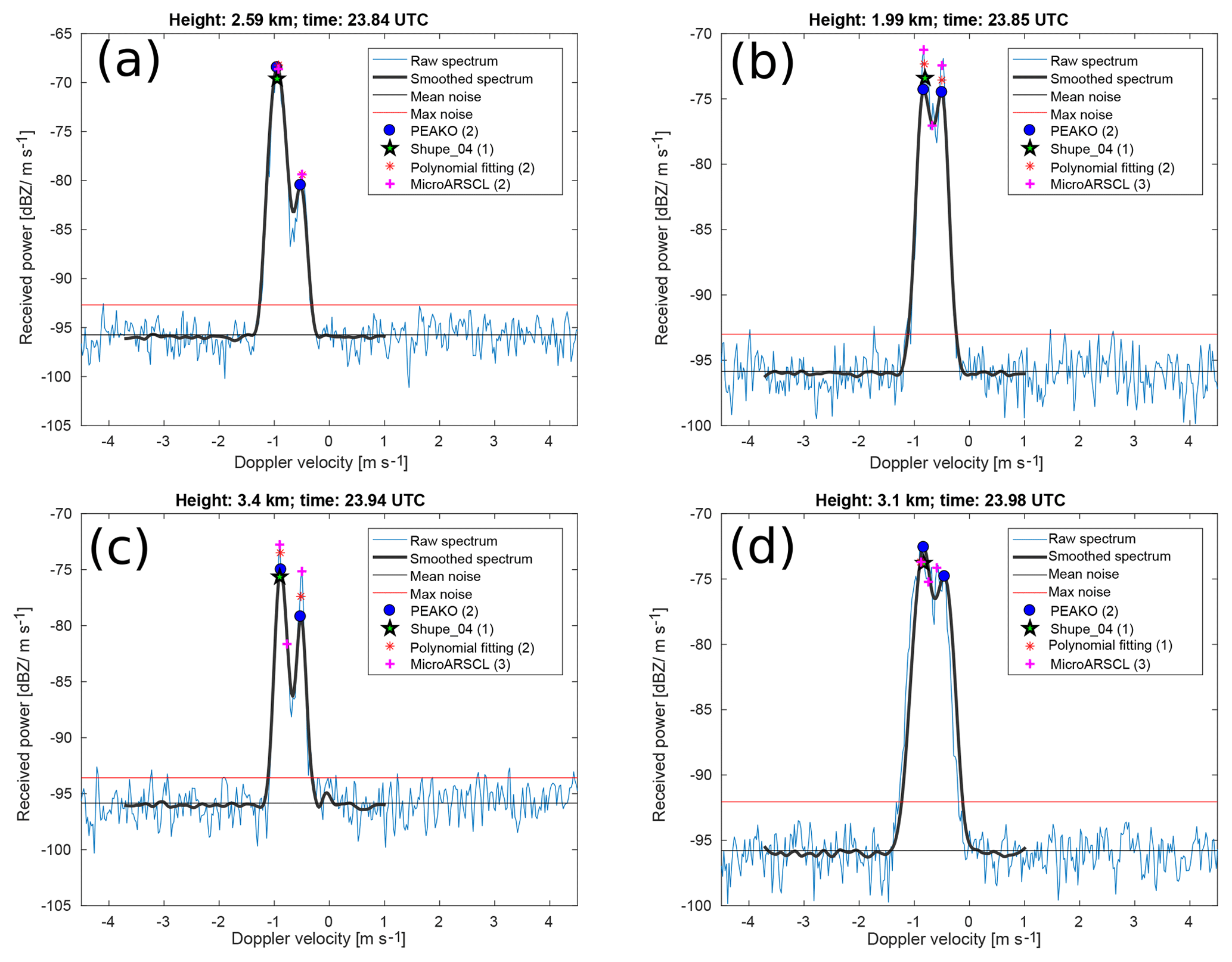
Figure C4Four example spectra picked from the case study on 7 February 2014, 23.75–24 UTC. Please note that the y axis scale is different for each of the spectrum plots.
To assess the influence of different smoothing schemes and spatiotemporal averaging space on the algorithm's performance, a sensitivity study was performed. Two smoothing methods available in MATLAB are the moving average and the locally weighted scatterplot smoothing (lowess) schemes. Lowess is very similar to loess with the difference that lowess utilizes a first-degree polynomial, which is fit to the data subset defined by span. We trained PEAKO in different configurations using the first training data set (Table 1). The PEAKO configurations tested were the following:
-
averaging over five spectra on a temporal scale and five spectra on a spatial scale, which results in an averaging timescale of 10 s and an averaging height of 150 m (the average spectrum is smoothed using the loess method).
-
omitting time–height averaging altogether prior to smoothing the spectra using loess.
-
keeping the spatiotemporal averaging fixed at the default of 16 s and 90 m but using moving average smoothing instead of the loess method.
-
keeping the spatiotemporal averaging scale fixed at the default and using lowess instead of loess.
The optimized parameters obtained after training PEAKO in each of the above-listed configurations were applied to the case study presented in Fig. 5. Figure D1 shows the results.
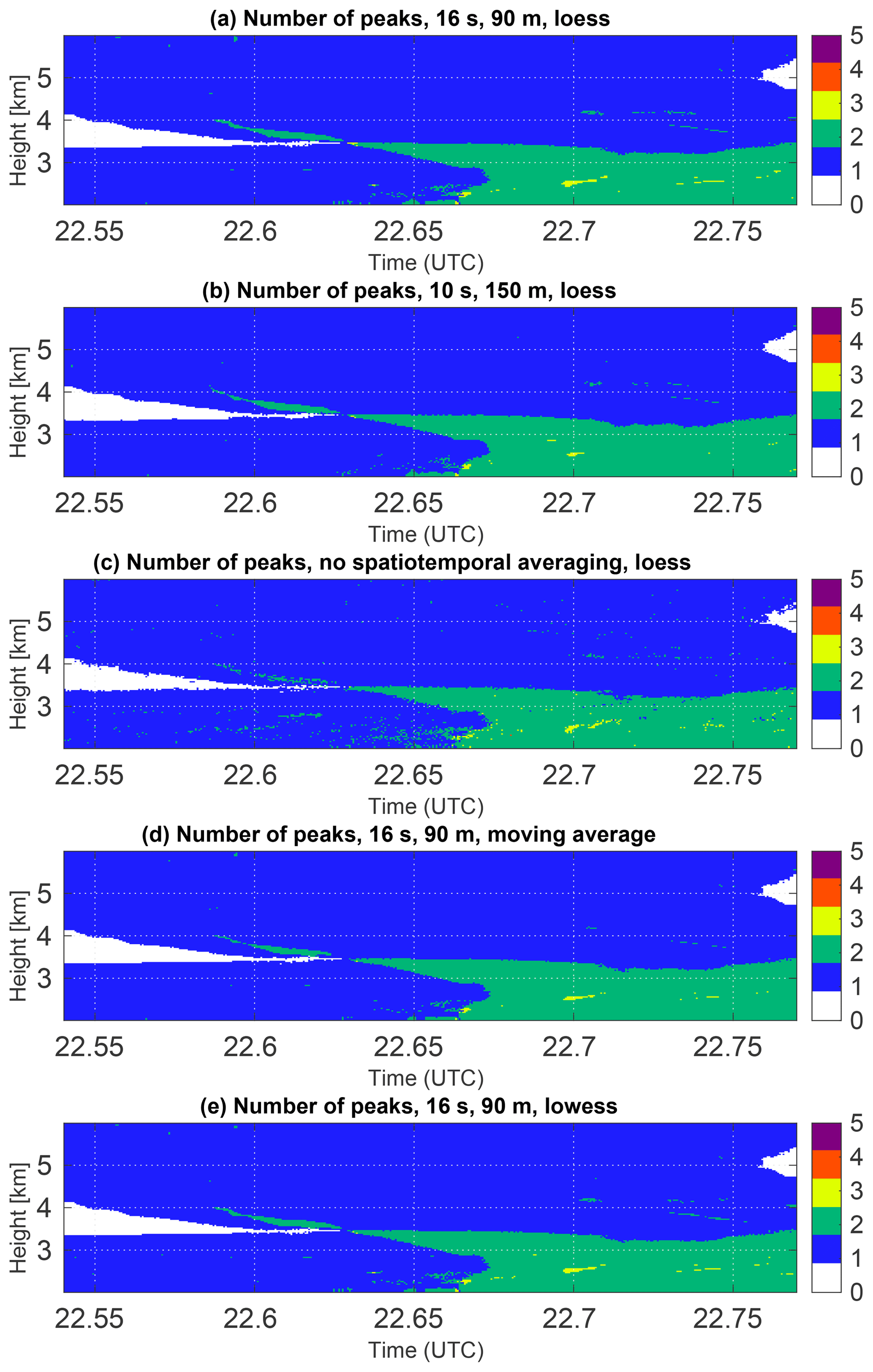
Figure D1Number of Doppler spectrum peaks detected by PEAKO in five different configurations for the selected case study on 21 February 2014 from 22.54 to 22.77 UTC, at 2 to 6 km altitude. (a–e) Number of peaks detected by PEAKO in the default configuration (16 s temporal and 90 m spatial averaging prior to loess); this plot is equivalent to Fig. 5a; number of peaks detected using 10 s temporal and 150 m spatial averaging followed by loess; number of peaks detected without time–height averaging prior to loess; number of peaks detected using 16 s and 150 m time–height averaging followed by smoothing using the moving average method; number of peaks detected using 6 s and 150 m time–height averaging followed by lowess.
The panels in Fig. D1 all display a similar pattern with respect to peak number. This is not surprising because the training process of PEAKO is the same for each of the methods, i.e., the three adjustable parameters are adjusted to obtain the best agreement with the human-created training data. A change in the spatiotemporal averaging scale towards more neighbors in height and fewer neighbors in time does not alter the result significantly. However, performing time–height averaging prior to smoothing at all is important as can be seen in the third panel in Fig. D1: if no spatiotemporal averaging is carried out before smoothing, the features detected by PEAKO become less coherent and more noisy. Figure D1d and e explore the effect of different smoothing schemes on the algorithm performance. Both moving average and lowess methods are able to reproduce the features detected by PEAKO in the default configuration only with some minor deviations.
HK, TV, and CP designed the PEAKO algorithm together. CP developed most of the MATLAB model code. HK and TV performed the data analysis and visualization and prepared the paper. EL contributed MicroARSCL data for the selected case studies.
The authors declare that they have no conflict of interest.
The authors thank the entire BAECC SNEX science team, the AMF2 team, and the SMEAR II staff for data acquisition and analysis. Thanks also to Annakaisa von Lerber of the Finnish Meteorological Institute for discussions on ground-based in situ data as well as Pavlos Kollias for discussions on peak-finding in cloud radar Doppler velocity spectra. Thanks to the Leibniz Institute for Tropospheric Research through which the student research position of Teresa Vogl has received funding from the European Union’s Horizon 2020 research and innovation program under grant agreement no. 654109.
This research has been supported by the DFG (grant no: GZ:KA 4162/1-1).
This paper was edited by Mark Kulie and reviewed by two anonymous referees.
Besic, N., Figueras i Ventura, J., Grazioli, J., Gabella, M., Germann, U., and Berne, A.: Hydrometeor classification through statistical clustering of polarimetric radar measurements: a semi-supervised approach, Atmos. Meas. Tech., 9, 4425–4445, https://doi.org/10.5194/amt-9-4425-2016, 2016. a
Bühl, J., Seifert, P., Myagkov, A., and Ansmann, A.: Measuring ice- and liquid-water properties in mixed-phase cloud layers at the Leipzig Cloudnet station, Atmos. Chem. Phys., 16, 10609–10620, https://doi.org/10.5194/acp-16-10609-2016, 2016.
Cornman, L. B., Goodrich, R. K., Morse, C. S., and Ecklund, W. L.: A Fuzzy Logic Method for Improved Moment Estimation from Doppler Spectra, J. Atmos. Ocean. Tech., 15, 1287–1305, https://doi.org/10.1175/1520-0426(1998)015<1287:AFLMFI>2.0.CO;2, 1998. a
Ermold, B., Eloranta, E., Michelsen, H., Garcia, J., Goldsmith, J., and Bambha, R.: High Spectral Resolution Lidar (HSRL), data set, https://doi.org/10.5439/1025200, 2014.
Hildebrand, P. H. and Sekhon, R. S.: Objective Determination of the Noise Level in Doppler Spectra, J. Appl. Meteor., 13, 808–811, https://doi.org/10.1175/1520-0450(1974)013<0808:odotnl>2.0.co;2, 1974. a, b, c, d
Kalesse, H., Szyrmer, W., Kneifel, S., Kollias, P., and Luke, E.: Fingerprints of a riming event on cloud radar Doppler spectra: observations and modeling, Atmos. Chem. Phys., 16, 2997–3012, https://doi.org/10.5194/acp-16-2997-2016, 2016. a, b, c, d, e, f, g, h
Kneifel, S., von Lerber, A., Tiira, J., Moisseev, D., Kollias, P., and Leinonen, J.: Observed relations between snowfall microphysics and triple-frequency radar measurements, J. Geophys. Res.-Atmos., 120, 6034–6055, https://doi.org/10.1002/2015jd023156, 2015. a, b, c, d, e, f, g, h, i, j, k, l, m, n, o, p, q, r, s, t
Kollias, P., Lhermitte, R., and Albrecht, B. A.: Vertical air motion and raindrop size distributions in convective systems using a 94 GHz radar, Geophys. Res. Lett., 26, 3109–3112, https://doi.org/10.1029/1999GL010838, 1999. a
Kollias, P., Albrecht, B. A., and Marks Jr., F. D.: Cloud radar observations of vertical drafts and microphysics in convective rain, J. Geophys. Res.-Atmos., 108, 4053, https://doi.org/10.1029/2001jd002033, 2003. a
Kollias, P., Miller, M. A., Luke, E. P., Johnson, K. L., Clothiaux, E. E., Moran, K. P., Widener, K. B., and Albrecht, B. A.: The Atmospheric Radiation Measurement Program Cloud Profiling Radars: Second-Generation Sampling Strategies, Processing, and Cloud Data Products, J. Atmos. Ocean. Tech., 24, 1199–1214, https://doi.org/10.1175/jtech2033.1, 2007. a, b
Kollias, P., Bharadwaj, N., Widener, K., Jo, I., and Johnson, K.: Scanning ARM Cloud Radars. Part I: Operational Sampling Strategies, J. Atmos. Ocean. Tech., 31, 569–582, https://doi.org/10.1175/jtech-d-13-00044.1, 2014. a
Kollias, P., Clothiaux, E. E., Ackerman, T. P., Albrecht, B. A., Widener, K. B., Moran, K. P., Luke, E. P., Johnson, K. L., Bharadwaj, N., Mead, J. B., Miller, M. A., Verlinde, J., Marchand, R. T., and Mace, G. G.: Development and Applications of ARM Millimeter-Wavelength Cloud Radars, Meteor. Mon., 57, 17.1–17.19, https://doi.org/10.1175/amsmonographs-d-15-0037.1, 2016. a, b
Komurcu, M., Storelvmo, T., Tan, I., Lohmann, U., Yun, Y., Penner, J. E., Wang, Y., Liu, X., and Takemura, T.: Intercomparison of the cloud water phase among global climate models, J. Geophys. Res.-Atmos., 119, 3372–3400, https://doi.org/10.1002/2013jd021119, 2014. a
Luke, E. P., Kollias, P., Johnson, K. L., and Clothiaux, E. E.: A Technique for the Automatic Detection of Insect Clutter in Cloud Radar Returns, J. Atmos. Ocean. Tech., 25, 1498–1513, https://doi.org/10.1175/2007JTECHA953.1, 2008. a, b
Luke, E. P., Kollias, P., and Shupe, M. D.: Detection of supercooled liquid in mixed-phase clouds using radar Doppler spectra, J. Geophys. Res.-Atmos., 115, D19201, https://doi.org/10.1029/2009JD012884, 2010. a
Mason, S. L., Chiu, C. J., Hogan, R. J., Moisseev, D., and Kneifel, S.: Retrievals of Riming and Snow Density From Vertically Pointing Doppler Radars, J. Geophys. Res.-Atmos., 123, 13807–13834, https://doi.org/10.1029/2018jd028603, 2018. a
Matthews, A., Isom, B., Nelson, D., Lindenmaier, I., Hardin, J., Johnson, K., and Bharadwaj, N.: Ka ARM Zenith Radar (KAZRGE), data set, https://doi.org/10.5439/1025214, 2014a.
Matthews, A., Isom, B., Nelson, D., Lindenmaier, I., Hardin, J., Johnson, K., and Bharadwaj, N.: Ka ARM Zenith Radar (KAZRSPECCMASKGECOPOL), data set, https://doi.org/10.5439/1025218, 2014b.
Oue, M., Kollias, P., Ryzhkov, A., and Luke, E. P.: Toward Exploring the Synergy Between Cloud Radar Polarimetry and Doppler Spectral Analysis in Deep Cold Precipitating Systems in the Arctic, J. Geophys. Res.-Atmos., 123, 2797–2815, https://doi.org/10.1002/2017jd027717, 2018. a, b
Petäjä, T., O'Connor, E. J., Moisseev, D., Sinclair, V. A., Manninen, A. J., Väänänen, R., von Lerber, A., Thornton, J. A., Nicoll, K., Petersen, W., Chandrasekar, V., Smith, J. N., Winkler, P. M., Krüger, O., Hakola, H., Timonen, H., Brus, D., Laurila, T., Asmi, E., Riekkola, M.-L., Mona, L., Massoli, P., Engelmann, R., Komppula, M., Wang, J., Kuang, C., Bäck, J., Virtanen, A., Levula, J., Ritsche, M., and Hickmon, N.: BAECC: A Field Campaign to Elucidate the Impact of Biogenic Aerosols on Clouds and Climate, B. Am. Meteorol. Soc., 97, 1909–1928, https://doi.org/10.1175/bams-d-14-00199.1, 2016. a
Praz, C., Roulet, Y.-A., and Berne, A.: Solid hydrometeor classification and riming degree estimation from pictures collected with a Multi-Angle Snowflake Camera, Atmos. Meas. Tech., 10, 1335–1357, https://doi.org/10.5194/amt-10-1335-2017, 2017. a
Radenz, M., Bühl, J., Seifert, P., Griesche, H., and Engelmann, R.: peakTree: A framework for structure-preserving radar Doppler spectra analysis, Atmos. Meas. Tech. Discuss., https://doi.org/10.5194/amt-2019-76, in review, 2019. a
Riihimaki, L. D., Comstock, J. M., Anderson, K. K., Holmes, A., and Luke, E.: A path towards uncertainty assignment in an operational cloud-phase algorithm from ARM vertically pointing active sensors, Adv. Stat. Climatol. Meteorol. Oceanogr., 2, 49–62, https://doi.org/10.5194/ascmo-2-49-2016, 2016. a
Shupe, M. D., Kollias, P., Matrosov, S. Y., and Schneider, T. L.: Deriving Mixed-Phase Cloud Properties from Doppler Radar Spectra, J. Atmos. Ocean. Tech., 21, 660–670, https://doi.org/10.1175/1520-0426(2004)021<0660:dmcpfd>2.0.co;2, 2004. a, b, c
Tan, I., Storelvmo, T., and Zelinka, M. D.: Observational constraints on mixed-phase clouds imply higher climate sensitivity, Science, 352, 224–227, https://doi.org/10.1126/science.aad5300, 2016. a
Verlinde, J., Rambukkange, M. P., Clothiaux, E. E., McFarquhar, G. M., and Elorant, a. E. W.: Arctic multilayered, mixed-phase cloud processes revealed in millimeter-wave cloud radar Doppler spectra, J. Geophys. Res.-Atmos., 118, 13199–13213, https://doi.org/10.1002/2013JD020183, 2013. a, b
Williams, C. R., Maahn, M., Hardin, J. C., and de Boer, G.: Clutter mitigation, multiple peaks, and high-order spectral moments in 35 GHz vertically pointing radar velocity spectra, Atmos. Meas. Tech., 11, 4963–4980, https://doi.org/10.5194/amt-11-4963-2018, 2018. a
- Abstract
- Introduction
- Data set description
- Methodology
- Results and discussion
- Conclusions and outlook
- Data availability
- Appendix A: Case study from 16 February 2014, 0.67–0.92 UTC (training data set 2)
- Appendix B: Case study from 21 February 2014, 23.01–23.10 UTC (training data set 3)
- Appendix C: Case study from 7 February 2014, 23.75–24 UTC (test data set 2)
- Appendix D: Sensitivity study on the effect of different smoothing schemes and spatiotemporal averaging scales
- Author contributions
- Competing interests
- Acknowledgements
- Financial support
- Review statement
- References