the Creative Commons Attribution 4.0 License.
the Creative Commons Attribution 4.0 License.
 | 02 Jun 2021
MICRU: an effective cloud fraction algorithm designed for UV–vis satellite instruments with large viewing angles
Steffen Beirle
Steffen Dörner
Marloes Gutenstein-Penning de Vries
Christoph Hörmann
Christian Borger
Simon Warnach
Thomas Wagner
Clouds impact the radiative transfer of the Earth's atmosphere and strongly influence satellite measurements in the ultraviolet–visible (UV–vis) and infrared (IR) spectral ranges. For satellite measurements of trace gases absorbing in the UV–vis spectral range, particularly clouds ultimately determine the vertical sensitivity profile, mainly by reducing the sensitivity for trace-gas columns below the cloud.
The Mainz iterative cloud retrieval utilities (MICRU) algorithm is specifically designed to reduce the error budget of trace-gas retrievals, such as those for nitrogen dioxide (NO2), which strongly depends on the accuracy of small cloud fractions (CFs) in particular. The accuracy of MICRU is governed by an empirical parameterisation of the viewing-geometry-dependent background surface reflectivity taking instrumental and physical effects into account. Instrumental effects are mainly degradation and polarisation effects; physical effects are due to the anisotropy of the surface reflectivity, e.g. shadowing of plants and sun glitter.
MICRU is applied to main science channel (MSC) and polarisation measurement device (PMD) data collected between April 2007 and June 2013 by the Global Ozone Monitoring Experiment 2A (GOME-2A) instrument aboard the MetOp-A satellite. CFs are retrieved at different spectral bands between 374 and 758 nm. The MICRU results for MSC and PMD at different wavelengths are intercompared to study CF precision and accuracy, which depend on wavelength and spatial correlation. Furthermore, MICRU results are compared to FRESCO (fast retrieval scheme for clouds from the oxygen A band) and OCRA (optical cloud recognition algorithm) operational cloud products.
We show that MICRU retrieves small CFs with an accuracy of 0.04 or better for the entire 1920 km wide swath with a potential bias between −0.01 and −0.03. CFs retrieved at shorter wavelengths are less affected by adverse surface heterogeneities. The comparison to the operational CF algorithms shows that MICRU significantly reduces the dependence on viewing angle, time, and sun glitter. Systematic effects along coasts are particularly small for MICRU due to its dedicated treatment of land and ocean surfaces.
The MICRU algorithm is designed for spectroscopic instruments ranging from the GOME to Sentinel-5P/Tropospheric Monitoring Instrument (TROPOMI) but is also applicable to UV–vis imagers like the Advanced Very High Resolution Radiometer (AVHRR), the Moderate Resolution Imaging Spectroradiometer (MODIS), the Visible Infrared Imaging Radiometer Suite (VIIRS), and Sentinel-2.
- Article
(33680 KB) - Full-text XML
- BibTeX
- EndNote


Clouds are the most clearly visible component of the atmosphere, both from the ground and from space. Their presence increases the shortwave albedo of the Earth and hence reduces the amount of solar radiation absorbed by the Earth. Clouds furthermore alter the radiative transfer (RT) within the atmosphere by effectively shielding the underlying atmosphere and surface from observation. This paper focuses on the influence of clouds on the measurement sensitivity for atmospheric trace gases retrieved from satellite observations in the UV and visible (UV–vis) spectral ranges. The largest portion of the Earth's surface is darker than overlying clouds. In this scenario, the measurement sensitivity – that is, the air mass factor (AMF) (Noxon et al., 1979; Solomon et al., 1987; McKenzie et al., 1991; Perliski and Solomon, 1993; Sarkissian et al., 1995; Rozanov and Rozanov, 2010; Deutschmann et al., 2011) – is decreased for trace-gas abundances below clouds and increased above (see, e.g. Wagner et al., 2003). For trace gases located within clouds, however, the influence of clouds depends on the cloud characteristics and trace-gas profiles. In any case, cloud properties need to be carefully constrained in order to achieve high accuracy in tropospheric trace-gas measurements from satellites (De Smedt et al., 2008; Liu et al., 2011; Barkley et al., 2012; Lorente et al., 2017). Boersma et al. (2004), for example, estimated the uncertainty in the tropospheric air mass factor for GOME measurements of nitrogen dioxide (NO2) due to uncertainties in the cloud fraction between 25 % and 30 % over large parts of North America, Europe, and southeast Asia, where most anthropogenic NO2 emissions occur.
Satellite retrievals of trace gases with high abundances in the boundary layer depend on the amount and properties of clouds within one satellite pixel. The effective cloud fraction (CF, c) is one measure to quantify cloud contamination. CF is defined by
based on the top-of-atmosphere (TOA) reflectance
with TOA radiance I, solar irradiance E0, and solar zenith angle ϑ0. This definition of c applies the independent pixel approximation (IPA), neglecting the influence of horizontal RT (Martin et al., 2002). Rmin and Rmax in Eq. (1) denote lower and upper thresholds corresponding to reflectances from cloud-free and completely cloudy pixels, respectively. Rmin depends on the reflecting properties of the surface and viewing geometry. Hence, an Rmin approximating the time dependency of the actual bidirectional reflectance distribution function (BRDF) is required for any geolocation in order to retrieve small CFs at high accuracy. In contrast, Rmax depends on cloud albedo. The cloud albedo depends on optical density and scattering properties, which can be described by an a priori cloud model, in addition to the observation geometry. Rmax may be empirically determined (e.g. Grzegorski et al., 2006; Lutz et al., 2016) or calculated using a radiative transfer model (RTM) (e.g. Wang et al., 2008). The Mainz iterative cloud retrieval utilities (MICRU) algorithm applies a Lambertian cloud model with a fixed albedo of 0.8 (e.g. McPeters et al., 1996; Stammes et al., 2008; Vasilkov et al., 2017), rendering Rmax depending on observation geometry alone.
Within tropospheric trace-gas retrievals, cloudy pixels are usually flagged by applying a threshold for c between 10 % and 30 %, and a high accuracy of c is required for the correction of cloud effects of the remaining pixels. Specifically, the accurate determination of Rmin is crucial to determine small CFs accurately. Rmin depends on the geolocation and time, and therefore maps of the lower threshold are needed. The Heidelberg iterative cloud retrieval utilities (HICRU), for example, derive background maps based on TOA reflectances using image processing techniques (Grzegorski et al., 2006; Grzegorski, 2009). In contrast, Koelemeijer et al. (2003) take Rayleigh scattering into account providing Lambertian-equivalent reflectivity (LER) maps. More sophisticated methods apply a complex BRDF accounting for the anisotropy of the surface reflectivity (Vasilkov et al., 2017; Lorente et al., 2018) or a geometry-dependent LER model (Vasilkov et al., 2018; Loyola et al., 2020).
Algorithms for the retrieval of background maps usually rely on completely cloud-free observations over a certain location. Here, we are interested in CFs of spectroscopic measurements. Compared to imager instruments, spectrometers are characterised by lower spatial but much higher spectral resolution. For example, the Visible Infrared Imaging Radiometer Suite (VIIRS) imager features 22 spectral channels at a resolution of approximately 400 m, whereas the spectrometer Ozone Monitoring Instrument (OMI) offers 1176 spectral channels at a nadir resolution of 13 km × 24 km (Schueler et al., 2002; Levelt et al., 2006; KNMI, 2019; de Graaf et al., 2016; Sihler et al., 2017). Based on this difference of spatial resolution, it becomes evident that the probability to obtain a completely cloud-free observation over a certain location is much higher for imagers than for spectrometers (Krijger et al., 2007). Therefore, background-reflectance-retrieving algorithms applicable to spectrometer data have to deal with much sparser statistics than those tailored for imagers.
Algorithms deriving cloud fractions from spectroscopic measurements feature different approaches for background maps. One of the first algorithms published for the Global Ozone Monitoring Instrument (GOME; Burrows et al., 1999) is the initial cloud fitting algorithm (ICFA), applying the global ETOPO5 digital elevation model (Kuze and Chance, 1994; Tuinder et al., 2004). Then, 7 years later, Koelemeijer et al. (2001) published the fast retrieval scheme for clouds from the oxygen A band (FRESCO), whose development continued as FRESCO+ (Fournier et al., 2006; Wang et al., 2008; TEMIS, 2021). Operational algorithms, like FRESCO+, apply background maps from auxiliary instruments in order to provide data directly after launch. The algorithms are then usually updated by implementing different background maps as the mission evolves. The background maps may be either supplied from spectrometers or images. FRESCO version 6, for example, applies imager data from the Medium Resolution Imaging Spectrometer (MERIS), resolving albedo gradients, e.g. over coastlines, much better than the spectrometer data (Popp et al., 2011). Kokhanovsky et al. (2009), on the other hand, interprets MERIS data using threshold techniques to derive cloud fractions for the Scanning Imaging Absorption Spectrometer for Atmospheric Cartography (SCIAMACHY; Bovensmann et al., 1999). FRESCO version 7 features another approach for the Global Ozone Monitoring Experiment 2 (GOME-2; Callies et al., 2000; Munro et al., 2006, 2016) by applying LER maps derived from GOME-2 itself (TEMIS, 2021; Tilstra et al., 2017b). Version 8 of FRESCO then applies a LER climatology derived from GOME-2 data by taking the viewing geometry into account. In contrast to FRESCO, the optical cloud recognition algorithm (OCRA) applies background maps derived in the RGB colour space (Loyola, 1998; Loyola et al., 2007; Lutz et al., 2016). In its third version, developed for GOME-2 and the Tropospheric Monitoring Instrument (TROPOMI; Veefkind et al., 2012), OCRA also accounts for degradation, viewing geometry dependence, and sunglint (Lutz et al., 2016). The fourth version of OCRA applied to TROPOMI is described by Loyola et al. (2018). For OMI, the first version of reprocessed OMI/Aura Level-2 cloud data product (OMCLDO2) (Stammes et al., 2008) uses albedo data from GOME (Koelemeijer et al., 2003) and Total Ozone Mapping Spectrometer (TOMS) (Herman and Celarier, 1997) for calculating effective cloud fractions, whereas OMCLDO2 version 2 (Veefkind et al., 2016) applies a LER database derived from OMI measurements themselves as published by Kleipool et al. (2008). It is preferred to apply background maps from the same sensor for cloud retrievals – like in Grzegorski et al. (2006), Veefkind et al. (2016), and Tilstra et al. (2017b) – in order to achieve higher CF accuracy especially at small CFs because radiometric properties and their dependence on viewing angles vary between sensors (e.g. Tilstra et al., 2012). This approach is especially suitable for scientific studies using data processed offline. However, operational CF processors require background obtained from auxiliary sensors because data from the same sensor are then not yet available.
Recent developments also focus on applying geometry-dependent background maps in CF algorithms. HICRU empirically derives lower thresholds for each of the three subpixels of GOME separately (Grzegorski et al., 2006). For instruments featuring wider swaths like OMI and GOME-2, the limitations of the LER surface model become more important (Vasilkov et al., 2017; Lorente et al., 2017, 2018; Fasnacht et al., 2019). Lorente et al. (2018) find biases in cloud fractions of up to 50 % between backward-scattering and forward-scattering geometries in the GOME-2 FRESCO and 26 % in the OMI OMCLDO2 cloud algorithms. Vasilkov et al. (2017) show that applying a geometry-dependent LER instead of a regular LER can lead up to a 50 % increase of the trace-gas column density over polluted areas. Furthermore, Vasilkov et al. (2018) compared CFs derived using geometry-dependent LER with those based on regular LER and found CF differences of up to 0.07, especially for small CFs. These absolute differences correspond to relative errors that have a significant impact on trace-gas retrievals. Aerosols, however, reduce the effect of the BRDF (Noguchi et al., 2015). These recent studies rely on BRDF information derived from Moderate Resolution Imaging Spectroradiometer (MODIS; Justice et al., 1998) measurements because similar information from spectrometers is still too sparse to derive all coefficients of, for example, the Ross–Li BRDF model (Wanner et al., 1995).
This paper presents a new method to derive a geometry-dependent lower threshold map from spectroscopic measurements. MICRU applies an empirical parameterisation of the geometry dependence in order to overcome the limitation of having sparse data per geolocation. MICRU derives the lower threshold as LER in contrast to its heritage algorithm (HICRU), which applies TOA reflectances directly. Hence, first-order atmospheric effects are accounted for. The remaining dependencies on the viewing angle, which may be either instrumental artefacts or physical, are modelled by a combination of a second-order polynomial and a reduced model for surface effects of land and sun glitter over ocean (Cox and Munk, 1954a; Harmel and Chami, 2013; Martin et al., 2016). It is noted that the idea of modelling the viewing angle dependence using a second-order polynomial is not new. For example, Várnai and Marshak (2007) used a second-order polynomial to model the mean optical thickness of inhomogeneous clouds in MODIS measurements.
In this study, we apply MICRU to GOME-2 data exemplarily. Unlike its heritage algorithm (HICRU), MICRU is applicable to almost arbitrary wavelength intervals in the UV–vis wavelength region. MICRU furthermore uses an RT model to reduce the influence of atmospheric scattering for the retrieval of Rmin. MICRU CFs are evaluated between 382 and 757.5 nm in order to investigate the spectral stability of the algorithm, the influence of the surface on CF accuracy, and the influence of spatial aliasing specific to GOME/GOME-2 instruments (EUMETSAT, 2015).
The MICRU algorithm has been developed as part of the cloud fraction verification activities for the S5P/TROPOMI (Veefkind et al., 2012) and Sentinel-5 satellite missions. The operational cloud fraction algorithm for Sentinel-5P (S5P)/TROPOMI is OCRA (Loyola et al., 2018), and FRESCO is an auxiliary cloud product used for selected level-2 products (Wang et al., 2008), respectively. A comparison between all three algorithms is performed in Sect. 3 after introducing MICRU in Sect. 2.
MICRU is designed to be applicable to UV–vis satellite sensors operating on Sun-synchronous orbits. In this study, we examine its applicability using GOME-2 data. This section first describes the required input data (Sect. 2.1) and the conversion between TOA reflectances R to the LER (Sect. 2.2). Section 2.3 then details the retrieval of Tmin maps. The calculation of Rmax is described in Sect. 2.4. Section 2.5 specifies the implementation of the MICRU algorithm, followed by a description of the data sets that MICRU results are compared to (Sect. 2.6).
2.1 Input data
2.1.1 GOME-2 data
The primary data used in this work are radiances measured by the GOME-2 instrument aboard the MetOp satellites. There are three essentially identical MetOp satellites in total: MetOp-A was launched in 2006, followed by MetOp-B and MetOp-C in 2012 and 2018, respectively. The MetOp satellites fly in a Sun-synchronous orbit with an Equator-crossing time around 09:30 LST (local solar time) (Munro et al., 2016). This study applies data from GOME-2A only as it features the longest uninterrupted time series at the time of the MICRU algorithm development.
GOME-2 has four spectral main science channels (MSCs) with a spectral resolution between 0.26 and 0.51 nm ranging between 240 and 790 nm. Each MSC band features 1024 spectral channels. This study uses GOME-2A MSC data collected between February 2007 and June 2013. Data before and after this period are discarded in order to avoid interferences from instrument startup and a change of the operational swath width, respectively (EUMETSAT, 2015). Furthermore, GOME-2 has two polarisation measurement devices (PMDs) covering a similar spectral range but at a much coarser spectral resolution: PMD-PP and PMD-SP measure the polarised intensity parallel and perpendicular to the slit of the spectrometer, respectively. Lang (2010) defines 15 discrete wavelength intervals for each PMD instrument. On 11 March 2008, the PMD band definitions of GOME-2A were updated to version 3.1 (EUMETSAT, 2015; Munro et al., 2016). Therefore, PMD data obtained before April 2008 are disregarded here in order to achieve a consistent PMD data set. All spectral data are contained in the level-1b (L1b) data (processor version 5.3) provided by EUMETSAT.
GOME-2 is a scanning spectrometer featuring a nominally 1920 km wide swath, which was reduced to 960 km in July 2013 (Munro et al., 2016). One swath consists of 32 MSC or 256 PMD pixels, respectively. One swath is divided into a forward and a backward scan. The scanner turns 3 times faster during the backward scan resulting in 3 times larger pixels, which are discarded altogether in the following. Hence, 24 MSC or 192 PMD pixels remain, respectively. At nadir, the nominal (that is, forward scan) MSC pixel size is 40 km × 80 km in along- and across-track directions, respectively. The PMDs feature an 8 times higher acquisition frequency, leading to a smaller pixel size of 40 km × 10 km. The illumination-observation geometry is defined by the solar zenith angle (SZA) θ0, the viewing zenith angle (VZA) θ, and the relative azimuth angle (RAA) ϕ as sketched in Fig. 1. The angles are defined at the pixel centre at the surface. It is noted that the along-track pixel size increases with increasing VZA due to the Earth's curvature. Hence, the pixel shape becomes trapezoidal (de Graaf et al., 2016; Sihler et al., 2017).
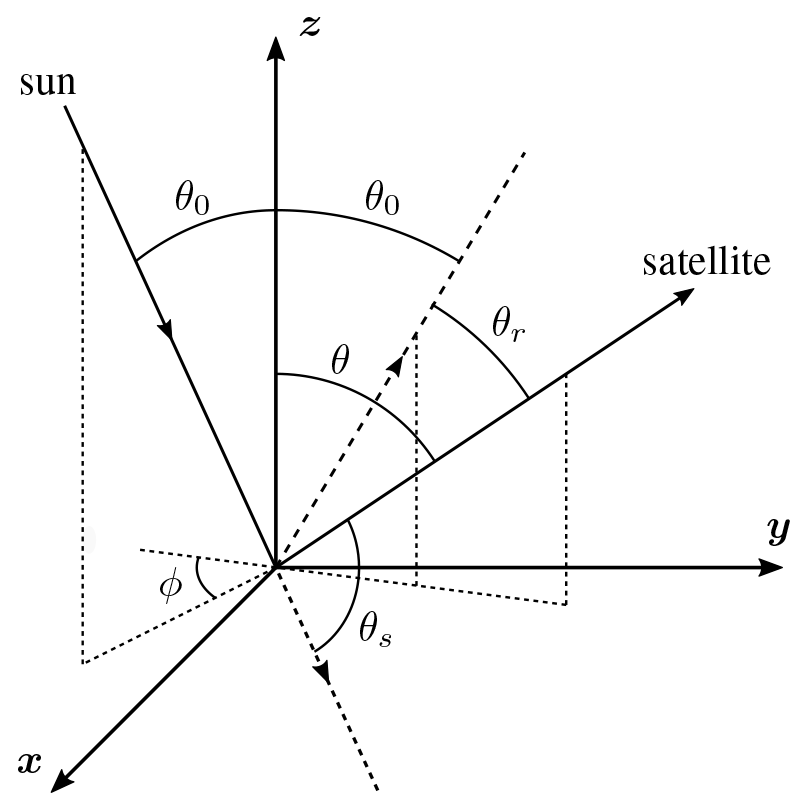
Figure 1Angle definition at the surface: solar zenith angle θ0, viewing zenith angle θ, relative azimuth angle ϕ, scattering angle θs, and reflected Sun angle θr. Zenith is towards z.
Table 1Definition of MICRU MSC channels k with spectral convolution kernels K centred at and width w. The kernels are either Gaussian (denoted G) or boxcar (denoted b) shaped. According to the spatial aliasing of GOME-2 (Fig. 3), channels 1, 4, 5, and 10 apply the same readout time as corresponding MSC or PMD channels in different bands.
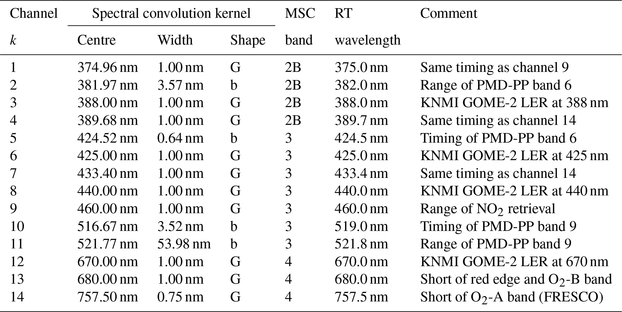
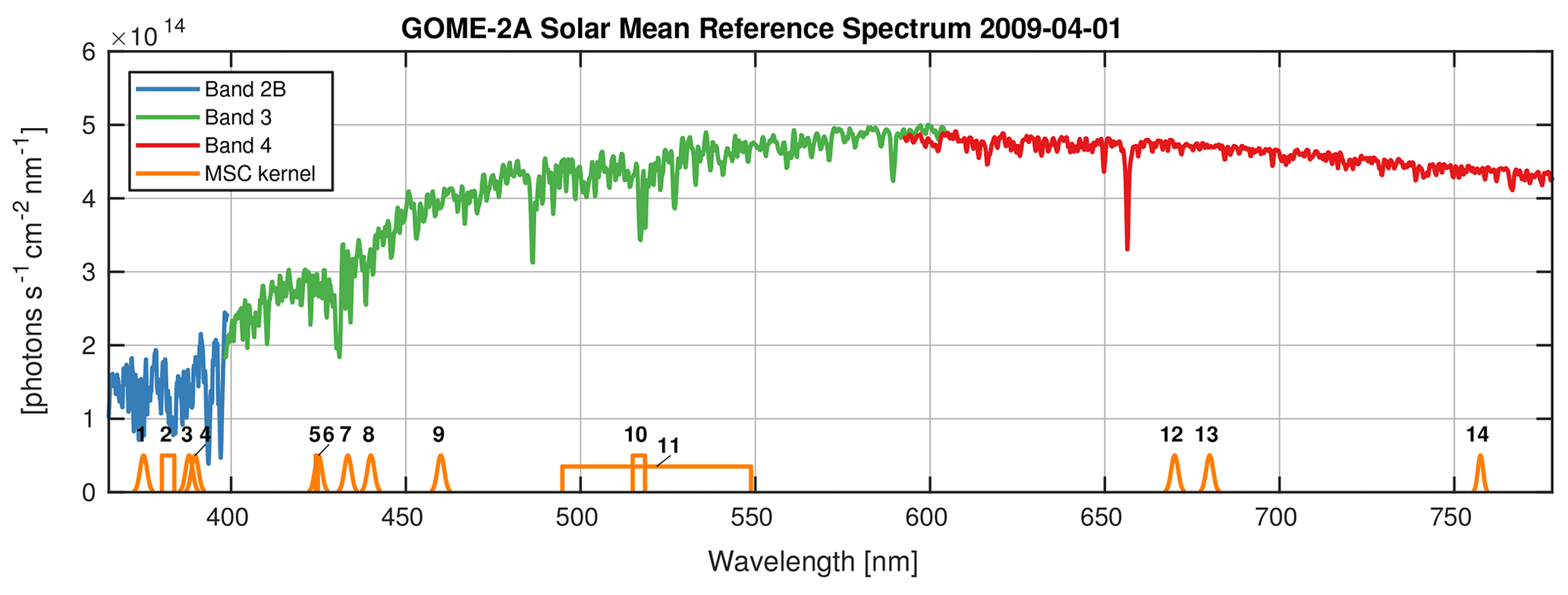
Figure 2Mean solar spectrum of GOME-2A MSC channel 2B, 3, and 4 recorded on 1 April 2009. Spectral convolution kernels Kk from Table 1 are plotted in orange. Note the small biases between overlapping bands due to different calibrations.
In the spectral domain, the MICRU algorithm is applied to 14 MSC and 16 PMD channels in order to assess the influence of systematic differences on the accuracy of c. In principle, the radiometric input required by MICRU may be integrated along any spectral interval, but it is beneficial to avoid significant absorption structures in order to minimise the influence of atmospheric absorptions. A dependence on the accuracy of the spectral calibration, which may not be optimal, is reduced by avoiding narrowband absorption features and Fraunhofer lines. Furthermore, broadband absorption by molecules and aerosols interferes with the inversion of the LER from measured R. Interferences may not be avoided completely in the UV–vis, but MICRU MSC channels are defined by minimising interferences from broad- and narrowband spectral features caused by Fraunhofer lines, inelastic Raman scattering (Grainger and Ring, 1962; Solomon et al., 1987, Ring effect), and molecular absorption by H2O, O2, and O4. The TOA reflectance Rk of MSC channel k is derived from the measured spectrum R(λ) by applying
where Kk is the convolution kernel of channel k. Kk indicates either Gaussian or boxcar convolution kernels with different widths as listed in Table 1 and depicted in Fig. 2. The MICRU PMD channels as listed in Table 2 are selected from predefined PMD bands (Lang, 2010).
Table 2Definition of MICRU PMD channels for PP and SP polarisation, respectively. PMD band definitions are compiled in Sect. 5.1.5 of EUMETSAT (2015) or Table 5 by Munro et al. (2016).

The convolution kernels for 14 MICRU MSC channels are manually defined in the range between 374 and 758 nm. Hence, CF results are available for a variety of spectral ranges with different atmospheric trace-gas absorptions. This is particularly important to improve collocation between CF and trace-gas measurement featuring different spatial sensitivities caused by spatial aliasing (EUMETSAT, 2015; Munro et al., 2016). Spatial aliasing is caused by the sequential detector readout in connection with the movement of the GOME-2 scanning mirror (Sihler et al., 2017). The comparison of MICRU results from MSC channels 2, 5, 10, and 11 allows the investigation of spatial aliasing. These channels furthermore allow us to compare the effect of spatial with spectral aliasing, which is due to differences in the spectral response of different channels. The horizontal arrows in Fig. 3 indicate MSC channels 2 and 5 matching the spectral sensitivity of the two PMD-PP/SP channel pairs 1/9 and 4/12, respectively. The vertical arrows indicate MICRU channels featuring the same acquisition time and hence minimising the spatial aliasing between them: MSC channels 2 and 10 correspond to PMD channels 1/9 and 4/12; MSC data acquired at the same time but in different bands are sampled by MSC channels 1 and 9 in bands 2B and 3, respectively, and MSC channels 4, 7, and 14 in bands 2B, 3, and 4, respectively. The correlation of MICRU CFs depending on spatial alignment is investigated in Sect. 3.3.3.
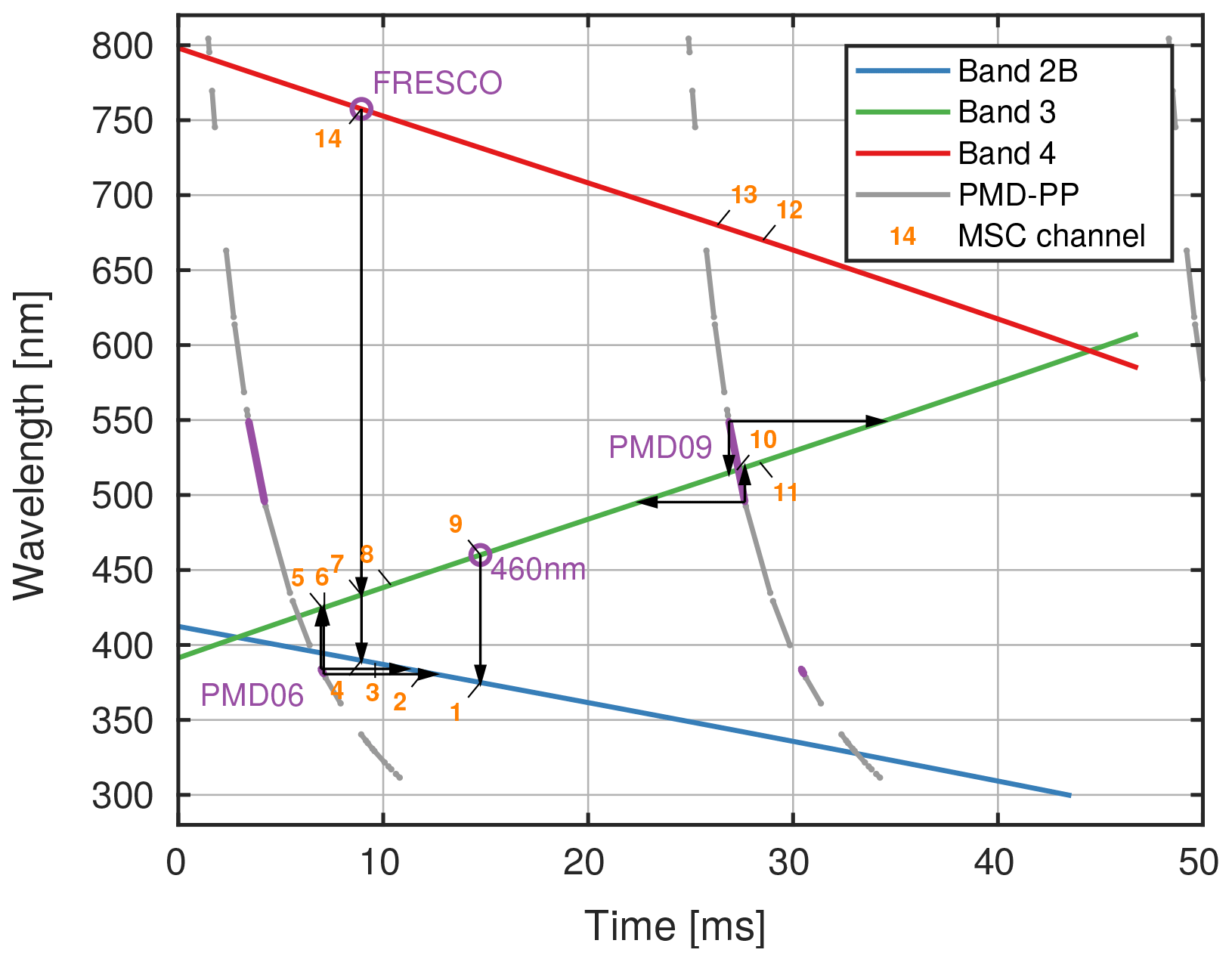
Figure 3Spatial aliasing of GOME-2 for MSC and PMD bands in time–wavelength space. Radiometric and spatial correlation is expected to be maximal at the respective intersections. Note that the PMD readout is faster (steep slope of gray lines) and at higher frequency compared to the MSCs. The second PMD readout (m=1) begins after 23.4375 ms (EUMETSAT, 2015). Horizontal and vertical black arrows indicate the spectral and temporal mapping between GOME-2 bands, respectively.
2.1.2 Auxiliary data for MICRU
The MICRU algorithm requires several external data sets listed in Table 3. Two different strategies of collocating these data to the GOME-2 observations are applied depending on the spatial resolution. Data provided at spatial resolutions significantly higher than the generic GOME-2 resolution are convolved with the respective average MSC and PMD point spread function (PSF), as depicted in Fig. 4. The average PSFs are derived from all forward scan pixel edges from one orbit of GOME-2A data at latitudes lower than 55∘. This approach simplifies the interpolation of auxiliary data on GOME-2 observations because a linear interpolation can be performed based on the GOME-2 pixel centre alone while providing still sufficient spatial accuracy. Data provided at coarser resolutions than GOME-2 are linearly interpolated based on the GOME-2 pixel centre without prior convolution.
Wessel and Smith (1996)NOAA (2018)USGS (2018)Hall and Riggs (2016)Cavalieri et al. (1996)Dee et al. (2011)Tuinder et al. (2020)Table 3List of external data sets applied in MICRU (see text for details).
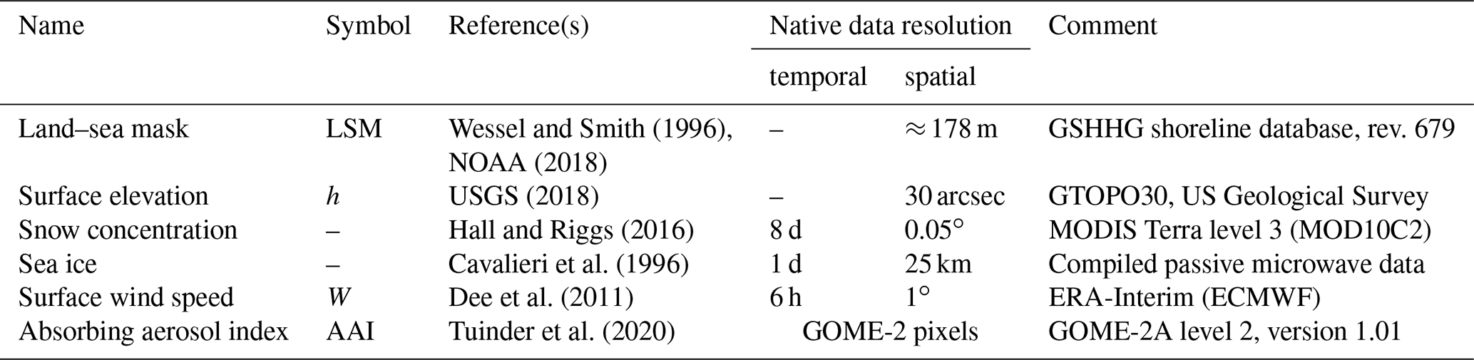
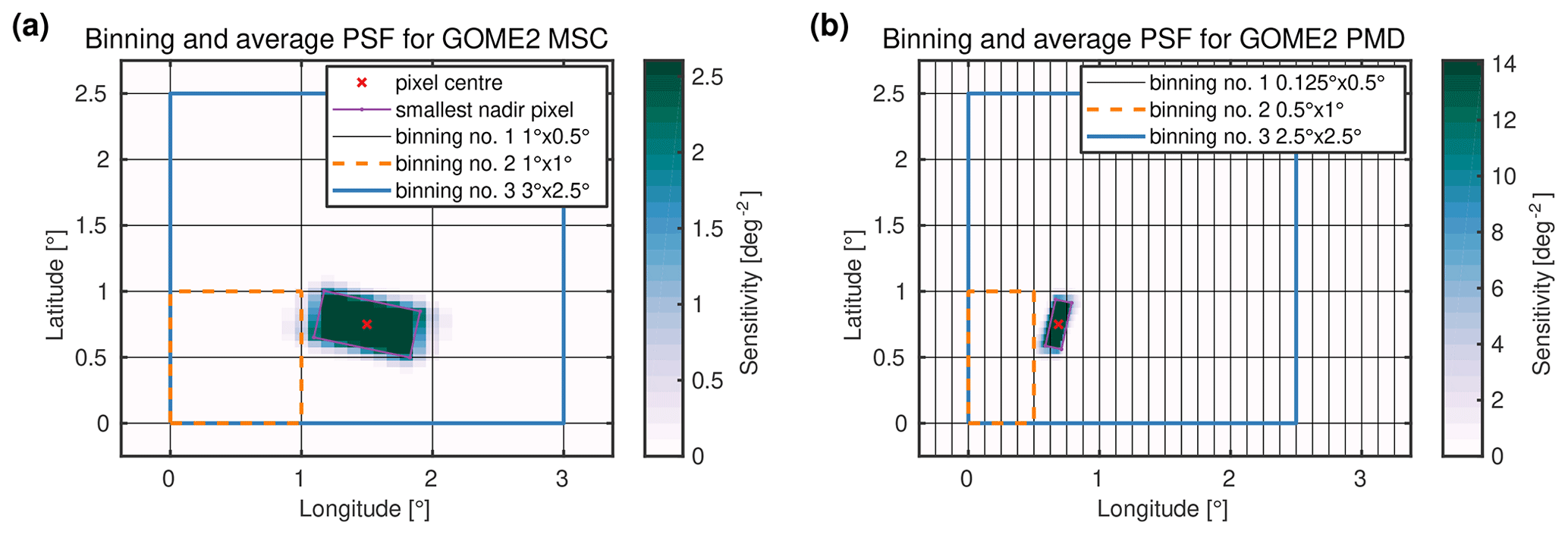
Figure 4Illustration of average MSC (a) and PMD (b) point spread functions (PSFs) used as convolution kernels for LSM, elevation, sea ice and snow concentration maps. The PSFs correspond to a nominal GOME-2 swath width of 1920 km. The highest resolutions for MSC and PMD lower threshold maps are 0.1∘ × 0.05∘ and 0.0125∘ × 0.05∘, respectively, and denoted as binning no. 1 as in Table 6.
MICRU features a separate Tmin parameterisation for measurements over land and ocean, respectively. An accurate description of the land and water transition is therefore crucial for the accurate interpolation of Tmin at coasts. An algorithm specifically developed for MICRU derives the fraction of water and land in each satellite pixel at high resolution. As input, the land–sea mask (LSM) compiled from revision 679 of the Global Self-consistent, Hierarchical, High-resolution Geography (GSHHG) shoreline database (Wessel and Smith, 1996; NOAA, 2018) is applied. The polygon data from intermediate GSHHG resolution neglecting polygons smaller in area than one GOME-2 pixel are first sampled at 0.1∘ × 0.05∘ and 0.0125∘ × 0.05∘ for MSC and PMD, respectively, and then convolved with the corresponding PSF (Fig. 4). The convolution yields a global map of fractional land cover ranging between 0 and 1 representing complete water and land coverage, respectively. Hence, Tmin values for land and ocean may be interpolated for each satellite pixel based on the convolved land cover map. The interpolated fractional land cover values are later also used for flagging (Sect. 2.5.3).
The second important input is the surface elevation h required for the inversion of the LER (Sect. 2.2). Elevations maps are inferred based on GTOPO30 raw data (USGS, 2018), which are averaged on a 0.05∘ × 0.05∘ grid, and convolved with a mean PSF sampled on the same grid resolution. Interpolation to GOME-2 resolution is again performed by applying nearest-neighbour interpolation.
Snow and sea ice data are queried to flag possible interferences from highly reflecting surfaces during post-processing (Sect. 2.5.3). Snow data are imported from MODIS Terra measurements with a similar Equator-crossing time of 10:30 LST in the descending node, similar to GOME-2. Hence, possible effects of different orbital parameters are supposed to be reduced. We used the 8 d composite MOD10C2 product (Hall and Riggs, 2016). Spatiotemporal interpolation uses the nearest-neighbour method based on spatially convolved 8 d maps as described above.
Sea ice data are provided by the National Snow and Ice Data Center (NSIDC) and integrate microwave measurements from different sensors (Cavalieri et al., 1996). These data have a native resolution of 25 km × 25 km, which is convolved using average PSFs on 0.1∘ resolution before merging to GOME-2. Data voids at the poles are filled with values from the nearest valid latitude. Unfortunately, there is no information on the sea ice concentration close to shores in the applied data set. This limitation leads to interferences at shores at high latitudes because GOME-2 pixels possibly affected by sea ice may not be filtered a priori.
Information on wind speed for the calculation of contributions from sun glitter is extracted from ERA-Interim data provided by the European Centre for Medium-Range Weather Forecasts (ECMWF) (Dee et al., 2011). ECMWF 10 m wind fields are used to parameterise sun glitter. As proposed by Ebuchi and Kizu (2002), the ECMWF wind fields are divided by a factor of 0.918 to approximate the wind speed at 41 ft (≈ 12.5 m) above the surface, which is required as input for the sun glitter model by Cox and Munk (1954a). This factor corresponds to a drag coefficient of 0.0015, assuming neutral stratification (Ebuchi and Kizu, 2002). ECMWF data are imported at 1∘ and 6 h spatial and temporal resolution, respectively. Spatially, nearest-neighbour interpolation is applied based on GOME-2 pixel centres.
Absorbing aerosol indices (AAIs) are also used to mask measurements potentially biased by aerosol effects (AAI > 2). For this purpose, AAI data inferred from GOME-2 measurements at both MSC and PMD resolutions are used (Tuinder et al., 2020). The reflectances used for the determination of the AAI at MSC resolution are centred at 340 and 380 nm. For the AAI at PMD resolution, PMD-PP bands 4 and 6 at 338 and 382 nm are applied, respectively. Hence, no interpolation is required to merge MICRU and AAI data.
2.2 RT calculations and inversion of LER
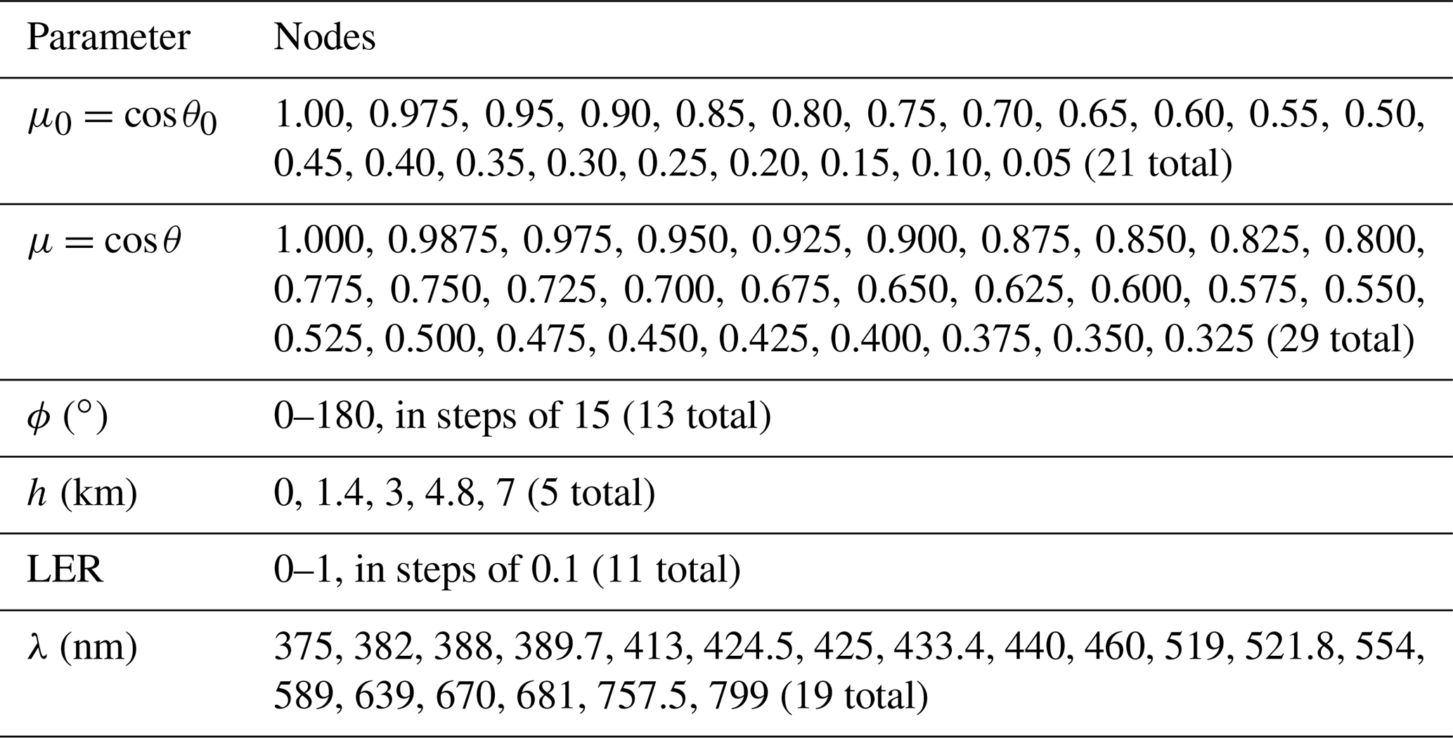
The conversion between surface LER and measured TOA reflectance R applies a look-up table (LUT) based on reduced reflectances . The LUT entries are pre-computed using SCIATRAN software version 3.7.1 (Rozanov et al., 2014; IFE-Bremen, 2018). The LUT has five dimensions: SZA, VZA , RAA, surface height h, and surface LER. Table 4 compiles the LUT nodes as well as the wavelengths applied as described in Sect. 2.1.1. It needs to be noted that the resolution of the LUTs in the LER direction may appear rather coarse. However, the difference of the obtained results compared to preliminary RT computations featuring a 10 times higher resolution was found to be < 0.001 in the UV and even 1 order of magnitude lower in the red spectral region. The LUT nodes in the SZA and VZA directions are defined in reduced angles μ0=cos θ0 and μ=cos θ, respectively, in order to provide more nodes at angles featuring larger gradients. The linear interpolation between the nodes is performed in θ0 and θ space, respectively, in order to increase numerical stability at nadir.
Table 4Definition of LUT nodes: reduced SZA μ0, reduced VZA μ, RAA ϕ, surface height h, and surface LER. The 5-D LUTs are calculated for 19 wavelengths λ.
The vector RT calculations are performed in spherical geometry based on a US standard atmosphere with 1013 hPa surface pressure at h = 0 m and accounting for atmospheric refraction. The surface is treated as a Lambertian reflector. The model accounts for molecular absorption by O3 and O4. The O3 column is fixed to 250 Dobson units (DU) in order to reduce the number of required input parameters. This simplification may affect MICRU retrievals within the ozone Chappuis band, most notably PMD channels 6 and 14, and, to a lesser extent, MSC channels 11 and 12. Preliminary results, however, showed that errors are on average negligible as the empirical approach of MICRU reduces the influence of systematic errors. Aerosols and Raman scattering are not included in the simulations.
From the LUT, the relation is interpolated for all observation geometries except for h < 0 km, which are tweaked to h = 0 km. is monotonic, and therefore can be readily inverted. We apply linear interpolation to infer .
2.3 Tmin retrieval
The Tmin MICRU algorithm requires a certain number of measurements in order to constrain its model parameters using observations not contaminated by clouds. For the description of the algorithm, we define a base set of measurements Ω0, which are spatially and temporally correlated. It is noted that Ω0 is a subset of all available measurements depending on grid resolution, measurement resolution, time period, surface structure, and cloud statistics. Section 2.5.1 describes the implementation of the subsetting process.
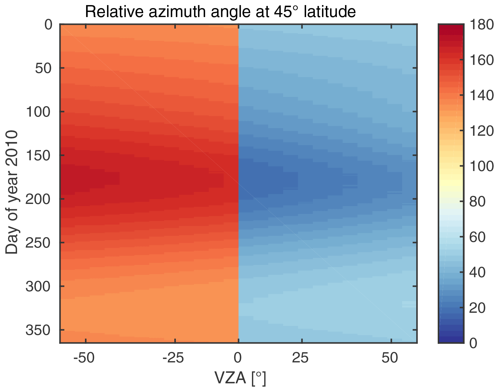
MICRU defines Tmin depending on the measurement geometry (θ0, θ, ϕ), geolocation, and time t. Tmin is not a true LER because it contains geophysical and instrumental information. This information is not separated within MICRU and will be treated simultaneously, as the ultimate goal is to determine a parameterisation of Tmin as accurately as possible. In general, it is not possible to parameterise Tmin in full (θ0, θ, ϕ) space due to the Sun-synchronous orbit of GOME-2 (Sect. 2.1.1). At every latitude, the dependencies of SZA and RAA on both VZA and time repeat annually. The dependence of SZA and RAA on VZA and time is exemplarily depicted for 45∘ N latitude in Figs. 5 and 6, respectively. It is therefore sufficient to parameterise the observation geometry (in each bin) by θ and t.
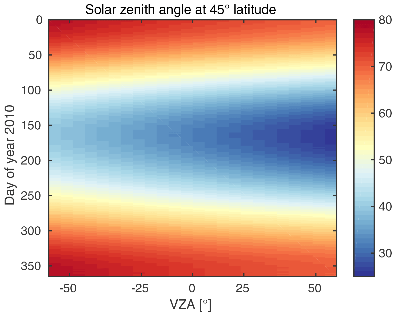
Figure 5SZA depending on time and VZA at 45∘ N latitude. Data bins correspond to 24 discrete forward scan pixels and individual days in the x and y directions, respectively. GOME-2A performs a Sun-synchronous orbit at a fixed inclination to the Sun. Hence, the SZA unambiguously depends on time, VZA, and latitude.
Ω0 typically contains a significant number of observations contaminated by clouds. Cloudy observations need to be filtered in order to retrieve a Tmin parameterisation based on cloud-free observations. Therefore, an iterative filter algorithm to find the lower accumulation point by Grzegorski et al. (2006) is presented in Appendix A. Compared to HICRU, however, the MICRU algorithm generalises from zero to four dimensions.
Tmin model
The MICRU Tmin model is
applying four independent variables (, , θs, and rg) and seven dependent variables (a0, at, ap, aa0, aa1, as, and ag), which are introduced in the following. Equation (4) is an empirical parameterisation accounting for actual and systematic effects of the lower threshold, which are not linearly independent in general.
Equation (4) applies normalised time and normalised VZA instead of t, and θ as independent model parameters to improve fit stability. Assuming t measures in units of days, we then define the normalised time:
measuring in units of years centred on t0. In the case of GOME-2A, t0 is chosen so that = 0 for 1 January 2010. θ measured in units of degrees and the normalised VZA,
ranges between −1 and 1.
The two further model parameters are the scattering angle θs, defined by
and the reflected Sun angle θr, defined by
Both angles are also illustrated in Fig. 1.
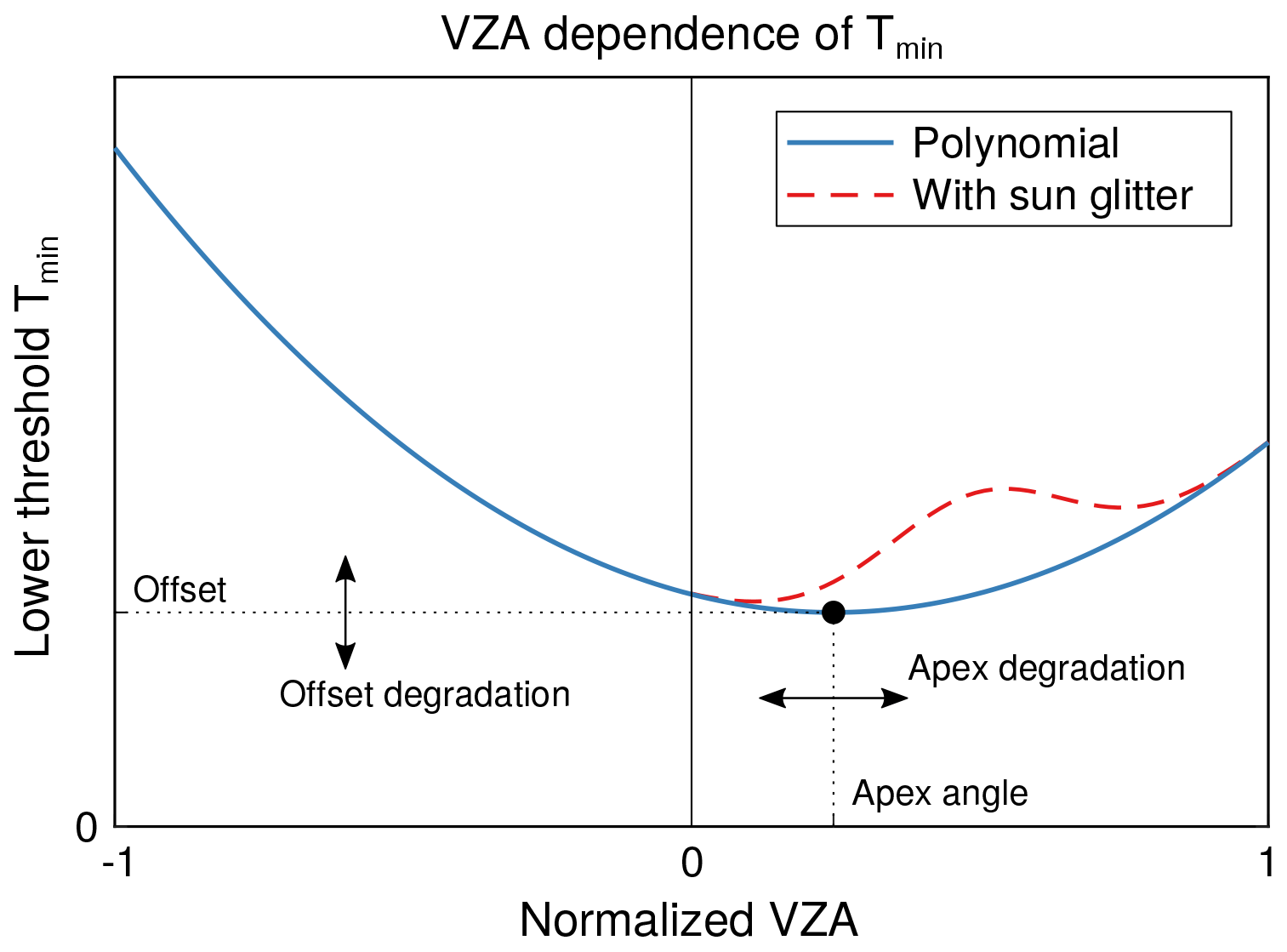
Figure 7A second-order polynomial parameterised by apex angle and curvature model systematic VZA dependencies of the lower threshold Tmin. Degradation may affect both apex angle and offset. The position, amplitude, and width of the sun glitter contribution depend on geometry and wind speed.
The right-hand side of Eq. (4) is the sum of the following terms.
-
The constant offset a0 accounts for the mean surface LER.
-
Residual line-of-sight dependencies are modelled by a second-order polynomial (Fig. 7), which is parameterised by the normalised apex angle and curvature ap:
-
Temporal degradation is assumed by a linear offset degradation factor at and the time-dependent normalised apex angle:
as indicated by the arrows in Fig. 7. Tests applying a second-order polynomial or an exponential to model degradation of GOME-2 MSC data were not successful. The former does not improve results significantly and the latter deteriorates the stability of the fit.
-
BRDF effects are modelled by an empiric cos θs term. Its inverse shows a similar behaviour to the Li dense kernel for closed canopy (Li and Strahler, 1992; Wanner et al., 1995) but does not require any further parameters. This term models the annual oscillations particularly visible at the western swath edge in Figs. 8d, e and 9d, e.
The cosine normalises the parameter improving the fit stability. As tests, we replaced the empirical term either with the precise Li dense kernels, a reduced cos θr term for surface effects, csc θs, or cos 2θs, but all of these tests resulted in less accurate surface fits and hence increased Tmin noise compared to our final choice.
-
The contribution of sun glitter on water surfaces is parameterised based on the isotropic sun glitter model suggested by Cox and Munk (1954a, b). This model was found to be sufficiently accurate for MICRU and, according to Zhang and Wang (2010), performs reasonably well compared to competing models in their study. We apply the glitter reflectance rg as provided in Eqs. (1)–(4), (9), and (15) in Zhang and Wang (2010). According to Cox and Munk (1954a), the mean square slope of the clean surface is
where W is the wind speed at 41 ft (≈ 12.5 m) above sea level, which is computed from 10 m wind speeds as described in Sect. 2.1.2. The index of refraction is set to n=1.34 (Blum et al., 2012). Hence, rg as illustrated in Fig. 7 is a function of θ0, θ, ϕ, and W.
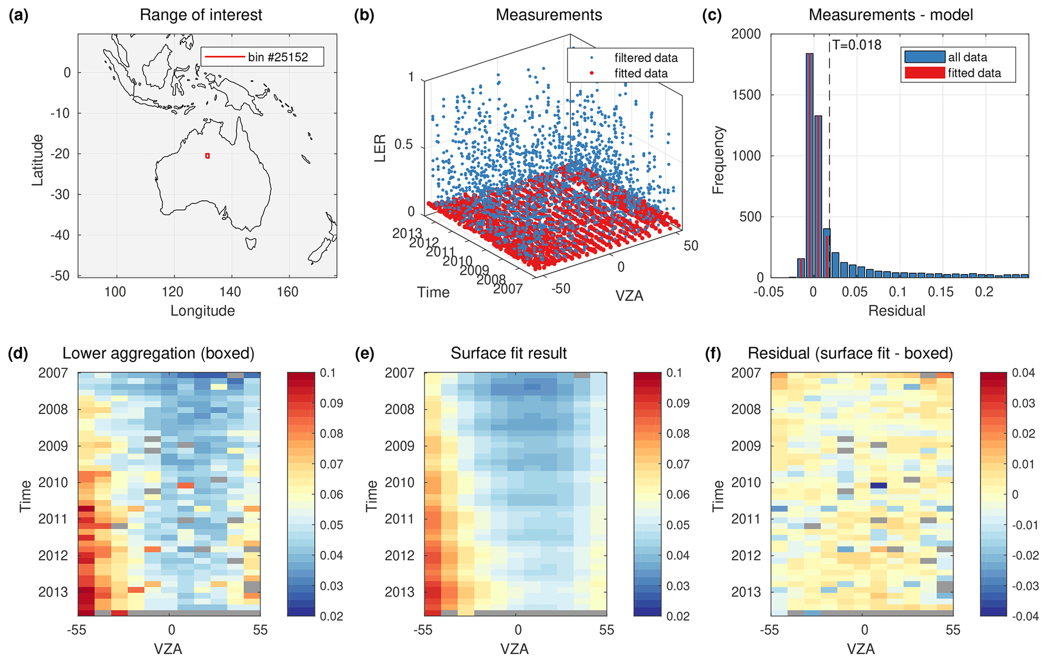
Figure 8Example surface fit for MSC channel 2 at 382 nm and applying binning no. 2 over Australia: (a) the bin of interest ranges from 131 to 132∘ E and from 20 to 21∘ S, (b) 3-D representation of measurement set Ω0 (blue) and finally fitted set ΩI (red), (c) frequency distribution of the fit residual, (d) lower accumulation point within each individual 0-D box, (e) surface fit result using model Eq. (4), and (f) difference between panels (d) and (e). The discretisation chosen for panels (d)–(f) displays a trade-off between accuracy and noise for the sake of clarity. Negative VZA denote the western half of the swath.
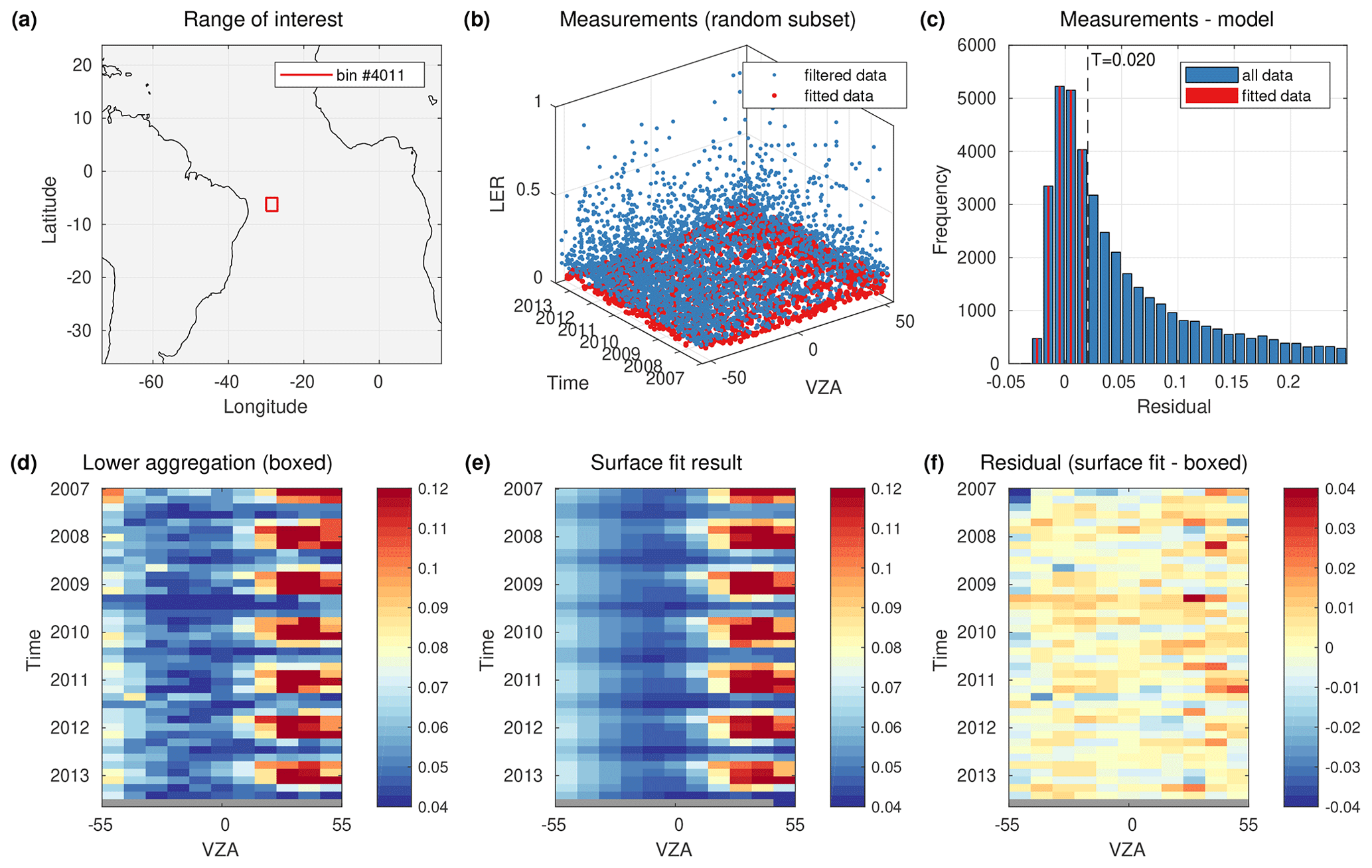
Figure 9Same as Fig. 8 but for MSC channel 10 at 516.7 nm and applying binning no. 5 over the equatorial Atlantic. The set of measurements ranges from 30∘ W to 27∘ E and from 7.55 to 5∘ S.
Table 5 summarises the Tmin model parameters and the bounds of the constrained fit. The parameters at and aa1 are constrained to 0 for MSC channels 12, 13, and 14, as preliminary evaluations showed that degradation can be neglected for these channels, which furthermore improved the signal-to-noise ratio. Clearly, the above model is a trade-off between accuracy and stability. Choosing a model based on more parameters would increase the accuracy of modelling the physical effects but degrade the stability of the fit limited by the number of cloud-free observations.
Table 5List of Tmin model parameters with initial values (β0) and parameter bounds of the constrained non-linear fit.
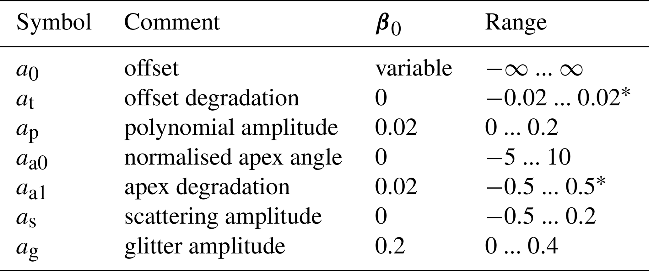
∗ Degradation constrained to 0 for MSC channels 12, 13, and 14.
2.4 Determination of Rmax
The upper threshold Rmax is defined as the reflectance of a Lambertian surface with an albedo of 0.8 located at 7 km altitude. This simple cloud model, which was adopted from McPeters et al. (1996) and Koelemeijer et al. (2001), improves applicability to retrievals building on MICRU cloud products because cloud correction algorithms in many trace-gas retrievals apply the same model (Vasilkov et al., 2017). Furthermore, the assumptions on cloud RT need to be consistent between cloud and trace-gas retrievals for AMF calculation. Volumetric clouds, on the other hand, are more complex to simulate and would require more parameters, which are unknown a priori.
Rmax is assumed independent of geolocation and time and calculated applying the look-up tables described in Sect. 2.2 and Table 4. A quantitative discussion of choosing Tmax = 0.8 as a cloud albedo for an Lambertian cloud model as an upper threshold is provided by Koelemeijer et al. (2001), Ahmad et al. (2004), and Stammes et al. (2008). As a consequence, however, very bright clouds exceeding Tmax = 0.8 will result in a MICRU CF > 1. Some CF algorithms normalise CF > 1 to 1, but MICRU rather provides these exceptionally high values as additional output.
It needs to be noted that instrumental degradation may introduce a systematic bias of the CF, which will be strongest for large CFs. Most importantly, for MICRU, the influence of the applied cloud model on the CF accuracy decreases with CF.
2.5 Implementation
The MICRU algorithm consists of several consecutive steps: import of data, RT simulation, merging of external data, determination of Rmin, determination of Rmax, and finally the computation of CF. The following subsections detail the implementation of the methods described above in the MICRU framework.
2.5.1 Geospatial subsetting
The Tmin algorithm (Sect. 2.3) requires a spatiotemporal subset of satellite measurements with a sufficient number of measurements. Section 2.1.2 describes how GOME-2 pixels are reduced to their centres. Hence, geospatial locations can be readily indexed and assigned to geospatial subsets. All MICRU computation refers to pixel centres rather than their actual area. This simplification takes advantage of the fact that the surface is scanned by almost identically shaped ground pixels over the evaluated measurement period, and therefore measurements with an identical pixel centre are congruent.
Temporally, larger subsets should be favoured over smaller ones unless there are significant changes of surface properties or the instrument response degrades much differently than considered in the model (Sect. 2.3). For example, for MSC binning no. 1, there are 400 equatorial bins over land with 15 or less measurements considered cloud-free by the Tmin retrieval despite applying a study period of 77 months. Longer time series increase the probability of including measurements not contaminated by clouds (Krijger et al., 2007).
Spatially, a very small geospatial interval would be beneficial in order to increase the correlation between measurement and collocated Tmin where the true surface is inhomogeneous. However, there is a trade-off because the probability of including enough cloud-free measurements decreases if the geospatial interval becomes too small. If there are not enough cloud-free measurements, the accuracy of the fit degrades. Furthermore, spatial subsampling can be avoided using spatial sampling intervals larger than the native resolution of the measurements defined by its PSF.
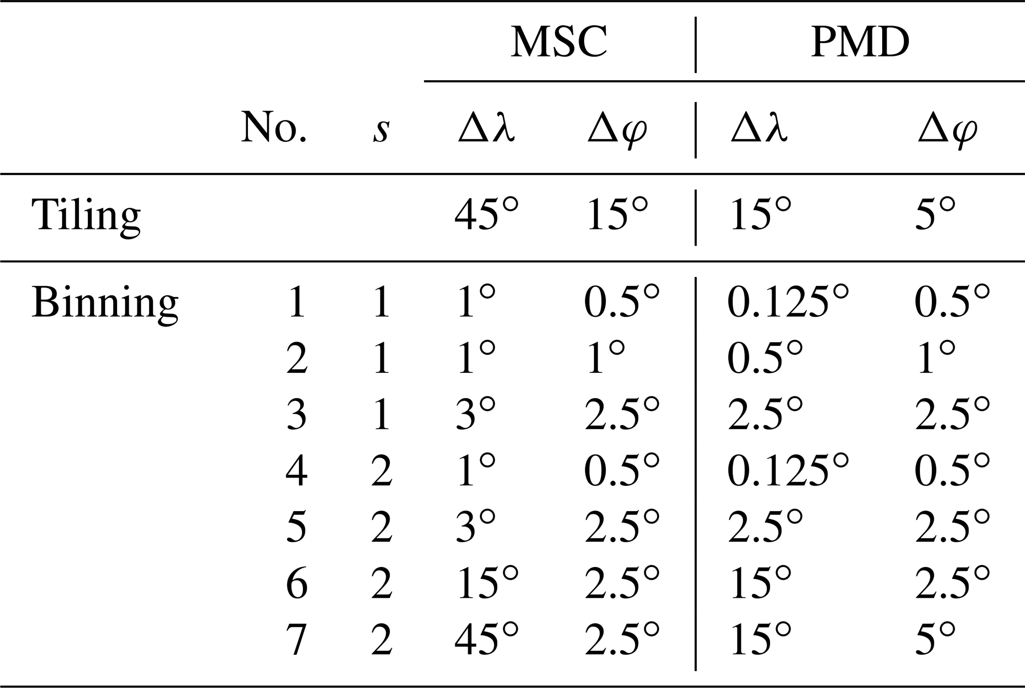
Within MICRU, the geospatial subsetting is called “binning”, which is performed on a longitude–latitude grid. Each binning corresponds to a global map at a different resolution. The Tmin retrieval is independently applied on each binning, whose definition distinguishes between measurements over ocean and land. The results are then merged to form complete parameterisations of Tmin for ocean and land surfaces independently. There are several advantages of this approach.
-
If, for some reason, the fit fails using the highest resolution, the parameterisation results from evaluation using larger bins may be used instead.
-
The bin dimensions can be adapted to the surface type: smaller and approximately quadratic over land; larger and less depending on longitude over ocean.
-
It enables independent parameterisations for the two different surface types. Hence, Tmin gradients at the coast can be mitigated.
Table 6 details and Fig. 4 illustrates the MICRU binnings for GOME-2 MSC and PMD evaluations, respectively. Figure 8a illustrates the dimension and location of bin 25152 of MSC binning no. 2.
Table 6Spacing of meridians (Δλ) and parallels (Δφ) for the definitions of tiling and binnings for MSC and PMD evaluations, respectively. Binning resolutions depend on surface type: land (s = 1) and ocean (s = 2).
The entire data set needs to be resorted with respect to geolocation instead of acquisition time for computational purposes. Therefore, input data are organised in geospatial “tiles” as defined in Table 6, which reduces the memory requirement for a process performing the iterative surface fitting per bin (Appendix A). Tiling furthermore enables parallel processing of MICRU on a cluster because each subprocess only requires a small portion of the observational data. Hence, scaling MICRU to sensors different from GOME-2 is straightforward by adjusting the tile resolution.
2.5.2 Tmin maps
The following filters are applied on the input data prior to the Tmin retrieval:
-
Filter measurement in ascending node to avoid ambiguities of the time- and latitude-dependent θ selection.
-
Filter viewing modes other than the nominal 1920 km swath (EUMETSAT, 2015). For example, this filter excludes nadir static and narrow swath orbits as well as data recorded after June 2013.
-
Filter SZA larger 85∘.
-
Filter data possibly affected by solar eclipses as defined in Appendix B of Tilstra et al. (2017a).
-
Filter times of instrumental malfunction as listed in EUMETSAT (2014).
-
Filter measurements with AAI > 2.
-
Filter measurements, which include neither > 90 % land nor > 90 % ocean.
-
Over ocean, filter measurements with θr < 8∘ (sun glitter).
Then, the Tmin algorithm (Sect. 2.3) is applied on the measurement tuples within each bin. Figure 8 illustrates the Tmin algorithm applied on MSC channel 2 for a 1∘ × 1∘ bin over Australia. Similarly, Fig. 9 illustrates the same on MSC channel 10 data at 516.7 nm over the Atlantic Ocean. This step is repeated for all binnings listed in Table 6 and all channels listed in Tables 1 and 2 for MSC and PMD, respectively. For diagnostic purposes, the number of iterations i, the number of included measurements N, the number of fitted measurements N∗, threshold τ, and residual statistics are intermediately stored alongside the fit result β for diagnostic purposes.
Tiled Tmin results are stitched together to form global maps for all binnings and channels. For each channel, the maps of different resolutions need to be merged in order to obtain two complete and unambiguous β maps, respectively: one for ocean and one for land. The steps of the merging process are detailed in Appendix B. Appendix C presents exemplary results for MICRU channel 2.
2.5.3 CF calculation and flagging
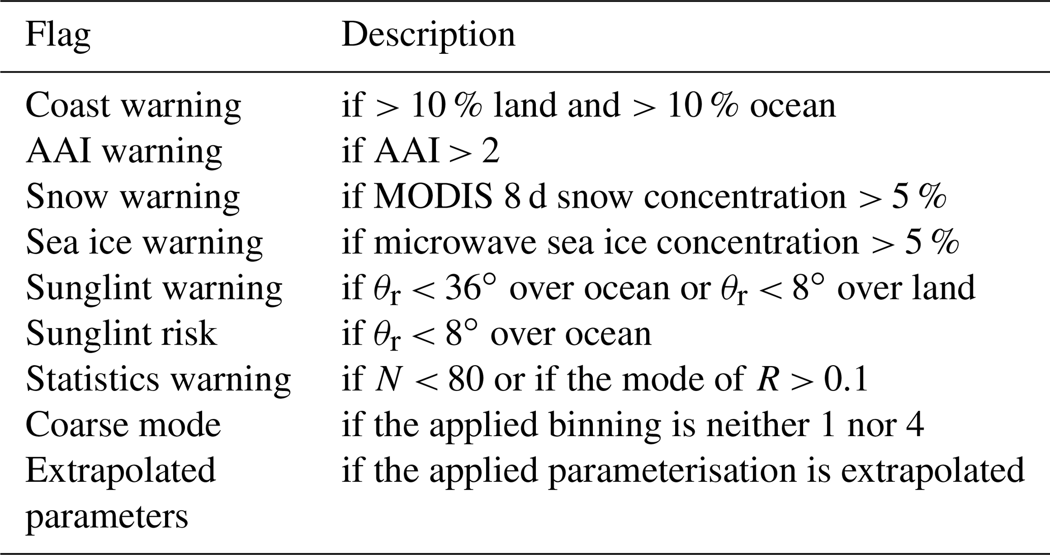
Once Rmin and Rmax are determined, c can be computed using Eq. (1) for all MICRU channels separately. The MICRU data set furthermore provides several quality flags listed in Table 7. MICRU MSC and PMD data are merged with three aliasing offsets (m=0, 1, 2) (Sect. 2.1.1) for the investigation of the spatial aliasing in Sect. 3.3.3.
Table 7Flags applied by the MICRU algorithm allowing for individual filtering.
2.6 Comparison data
For GOME-2 MSCs, FRESCO+ cloud fractions evaluated at the O2-A band are widely used (Wang et al., 2008; TEMIS, 2021). In this study, three different versions of the FRESCO cloud fractions are applied in order to study the particular differences with respect to background map generation and residual VZA dependence:
- FRESCO L1b
-
denotes the CF data shipped with the L1b files from EUMETSAT, also denoted FRESCO version 6. This FRESCO version applies a background map compiled from MERIS measurements over land and GOME-1 surface LER over ocean (Popp et al., 2011; Tilstra et al., 2017b).
- FRESCO v7
-
is the first FRESCO version applying a background LER map derived from GOME-2 measurements themselves (Tilstra et al., 2017b).
- FRESCO v8
-
is the most recent version applying a directional LER database compiled from GOME-2 measurements. The resolution at the coast and over specific regions is increased to reduce interference from different surface types within one GOME-2 pixel (Wang et al., 2018).
FRESCO L1b data of the entire evaluation period are included in this study. For FRESCO v7 and v8, however, comparisons to MICRU are limited to selected months. For FRESCO v7, it is January, April, July, and October 2010. For FRESCO v8, it is January to December 2010 plus April 2007 and 2013 (see Fig. 24b and c). The applied FRESCO products do not correct for interferences with sun glitter. It is furthermore noted that MICRU data are ignored in the comparisons in Sect. 3.4 if respective OCRA/FRESCO data are invalid.
The second batch of comparison data are OCRA cloud fractions inferred from GOME-2 PMD measurements described by Lutz et al. (2016). In its actual version (3.0), OCRA is mainly developed as the operational CF product for the S5P/TROPOMI mission (Loyola et al., 2018). In contrast to FRESCO, OCRA applies an empirical correction scheme for the sunglint effect (Lutz et al., 2016). OCRA CFs are officially provided at PMD resolution and are therefore suited to be compared directly to MICRU PMD results. OCRA results mapped to MSC resolution are denoted OCRA MSC. OCRA, however, does not assume a constant cloud albedo of 0.8 as the upper threshold, resulting in systematic differences between both products. We therefore introduce scaled OCRA results as a third OCRA data set. The scaling performed requires the cloud albedo CAROCINN retrieved by the retrieval of cloud information using neural networks (ROCINN) algorithm (Loyola et al., 2007, 2011, 2018), which is therefore only available at MSC resolution. We define the scaled OCRA CF CFOCRA_fixed_albedo by
denoted as “OCRA_fixed_albedo” below.
The selected cloud products define the upper threshold differently. FRESCO applies a Lambertian (or reflecting) cloud model – like MICRU – and OCRA applies a colour space approach for the upper threshold (Wang et al., 2008; Lutz et al., 2016). Furthermore, the treatment of extreme CFs significantly differs between MICRU, FRESCO, and OCRA. Both FRESCO and OCRA provide normalised CFs, which means that CFs do not linearly scale with reflectance. OCRA, for example, normalises CF < 0 to 0 and CF > 1 to 1. For FRESCO, normalisation schemes defer between versions: FRESCO L1b sets CF < 0 to 0. For CF > 1, all FRESCO versions vary the cloud albedo to improve convergence. In contrast, MICRU does not apply any normalisation by default, leading to an unlimited CF distribution. We define “cropped” subsets of data: CFs < 0 are set to 0 and CFs > 1 are omitted from statistical comparisons (Sect. 3.4) in order to avoid systematic bias from different normalisation strategies. It shall be noted that both normalisation and cropping lead to biased mean results. These biases propagate into trace-gas retrievals if normalised CF data are applied.
Finally, measurements by the AVHRR/3 (Advanced Very High Resolution Radiometer version 3) instrument are applied as independent measurements for the detection of clouds from the MetOp satellite (Cracknell, 1997; NOAA, 2021; EUMETSAT, 2011). AVHRR is an imager with six spectral channels centred between 630 nm and 12 µm. The spatial sampling of GOME-2 and AVHRR is detailed by Sihler et al. (2017). In this study, AVHRR data of bands 1, 2, and 3a are applied to produce RGB false colour images. Furthermore, an artificial AVHRR cloud mask is constructed, where an AVHRR pixel is assumed cloudy if either the albedo test, the T4-T3 test, or the T4-T5 test indicates a cloudy scene (see EUMETSAT, 2011).
This section starts off with results from the Tmin retrieval (Sect. 3.1) and a comparison between MICRU, FRESCO, and OCRA based on single, cloud-free swaths (Sect. 3.2). Subsequently, statistical ensembles are applied to intercompare MICRU CF results (Sect. 3.3) and to evaluate differences between the three CF algorithms (Sect. 3.4).
Studies on monthly statistics exclude data where
-
SZA ≥ 84∘,
-
latitudes ≥ 55∘,
-
MODIS snow concentration > 2 %,
-
AAI > 2,
-
the sunglint risk flag is raised, or
-
the coast warning is raised (exception: average maps)
in order to reduce interferences.
3.1 Tmin retrieval
Figure 8 illustrates the input measurements and output results of the Tmin retrieval (Sect. 2.3) by applying MSC channel 2 at 382 nm and binning no. 2 over continental Australia. The blue dots in Fig. 8b denote the input data, omitting scattering angle θs and glitter reflectance rg dimensions for the sake of clarity. Figure 8d shows a matrix of lower aggregation points of LER retrieved independently in discrete boxes defined in the t–θ plane. The lower aggregation points are retrieved with the same τ resulting from the surface fit but without parameterisation. The matrix reveals an increasing trend with time and a significant VZA dependence. The iterative surface fitting result using the same data (Fig. 8e) shows a similar but much smoother result due to improved statistics by combining the information from all measurements and applying a parameterised surface model. Figure 8f shows the difference between boxed and fitted results, indicating average deviations much smaller than 0.04. There are, however, small systematic deviations towards the edges indicating a slight overestimation of Tmin at the beginning of the sensing period (2007) and at large VZAs, and slight underestimation at the end of the period (colder colours for 2013). The histogram of the residual R of LER measurements and modelled Tmin is plotted in Fig. 8c using the respective colours as in Fig. 8b. Measurements applied for the final iteration of the surface fit peak between −0.01 and 0, for which a final threshold of τ = 0.018 is applied.
Figure 9, in contrast to Fig. 8, illustrates the application to another MSC channel at 516.7 nm and surface type ocean. Compared to Australia, the fraction of fitted measurements is significantly lower due to a higher probability for clouds. The smaller fraction of fitted measurements is also indicated by a less pronounced peak in the histogram (Fig. 9c). There is a significant contribution of sun glitter, which is visible by the annually appearing red areas at positive VZA in Fig. 9d and e. The scatter in Fig. 9f collocated with the regions affected by sun glitter is probably due to poor statistics when calculating the boxed comparison results. The LER in the first, western-most column of boxes seems to be biased low, of the order of 0.01, compared to other viewing angles.

Figure 10Detailed fit results from surface of three GOME-2 bands measured over Australia (cf. Fig. 8a), comparing the fit results with measurements selected from the beginning (blue dots) and the end (green dots): (a) MSC channel 2, the fit results (red lines) correspond to Fig. 8f, (b) for PMD-PP, and (c) for PMD-SP. Note the significant differences between the residual VZA dependence and the trends of three GOME-2 bands measuring at the same wavelength of 382 nm. Note that reflectance measurements below the red line will later result in negative CFs.
Figure 10 investigates trends of the VZA dependence for the three GOME-2 channels (MSC, PMD-PP, and PMD-SP) but same spectral region, respectively. Figure 10a corresponds to the first and last rows in Fig. 8d/e, indicated by blue and green dots, respectively. Circled dots correspond to the red dots in Fig. 8b. The red lines correspond to the fit results shown in 8e. Figure 10a reveals a lower threshold increasing with time (≈ 0.02 in total) and a time-dependent VZA dependence affecting apex VZA and curvature. Figure 10b and c illustrate the temporal behaviour of the corresponding PMD-PP and PMD-SP measurements. For PMD-PP, the VZA dependence and its degradation is smallest compared to the other channels. PMD-PP, however, features a significantly larger overall trend compared to PMD-SP in Fig. 10c. For PMD-SP, the overall trend is small, but the VZA dependence degrades significantly more than MSC channel 2.
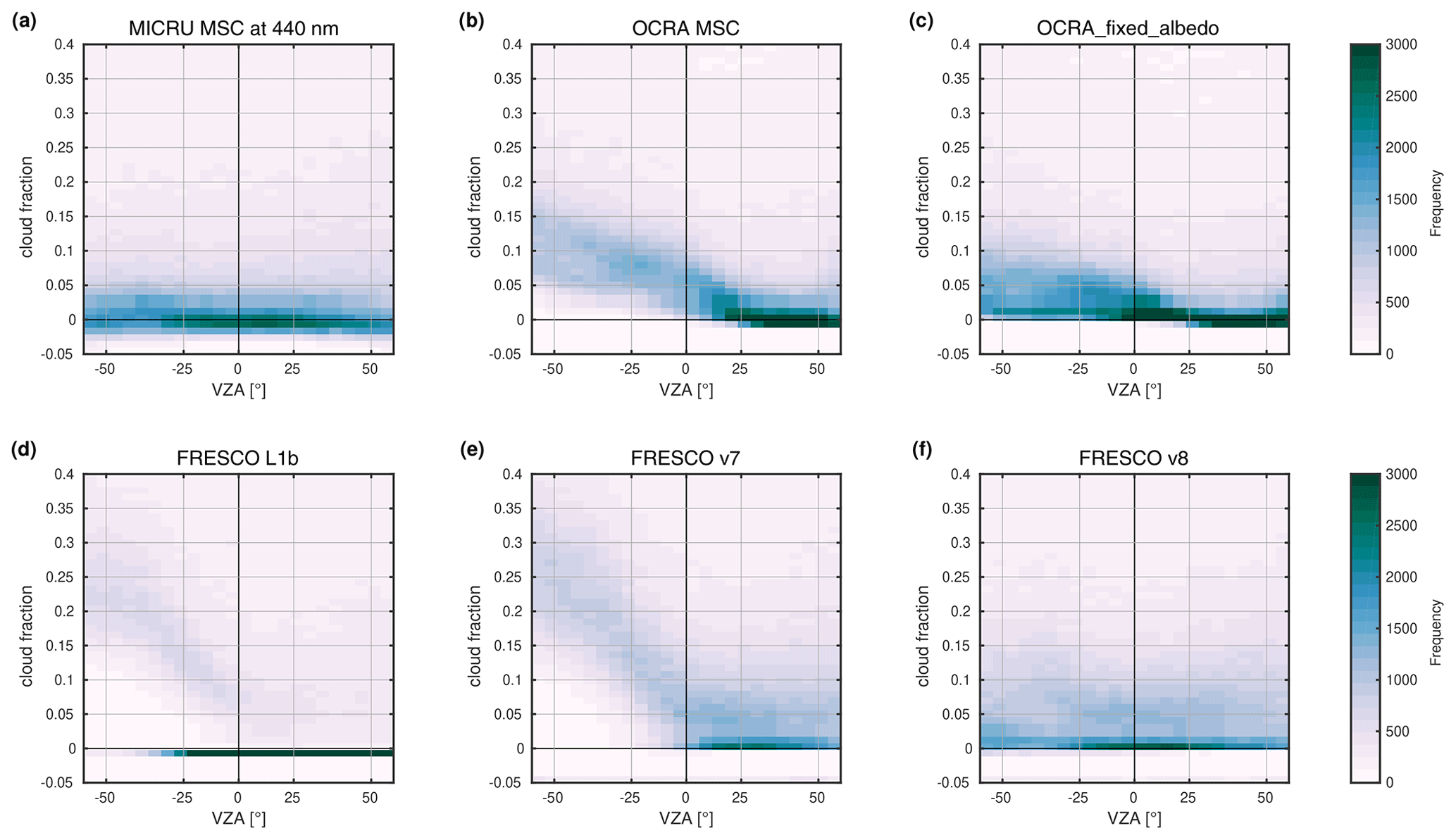
Figure 11Comparison of viewing angle dependence of small CFs over land between the 55∘ parallels: (a) MICRU MSC at 440 nm, (b) OCRA MSC, (c) OCRA_fixed_albedo, (d) FRESCO L1b, (e) FRESCO v7, and (f) FRESCO v8. Statistics are based on April 2010 data.
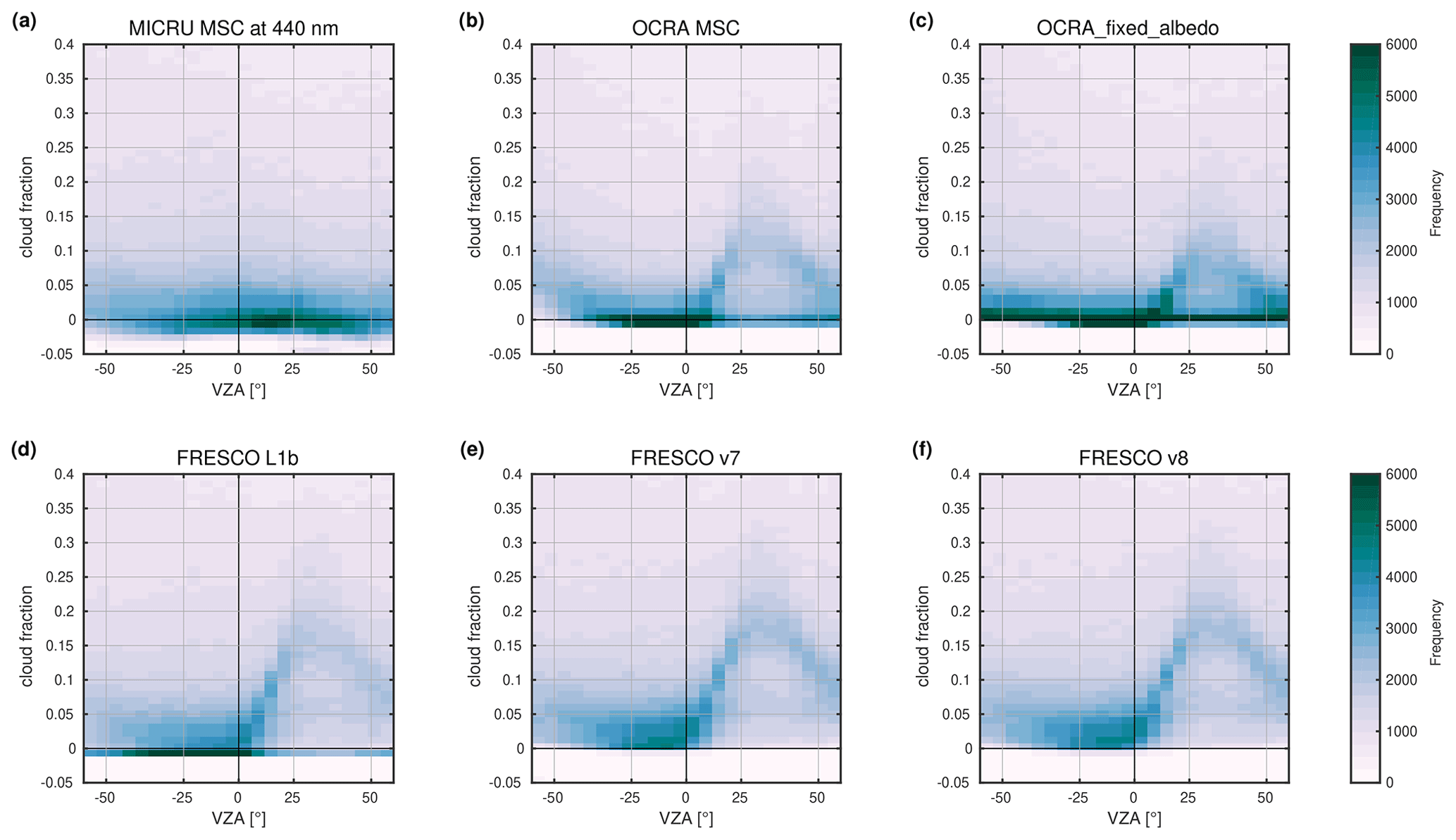
Another estimate of the residual VZA dependence may be assessed by analysing the cross-track dependence of the lower CF accumulation point displayed in Figs. 11a and 12a for land and ocean surfaces, respectively. Over land, the small CFs accumulate between −0.02 and 0.03 almost evenly over the entire swath. Over ocean, small CFs are slightly more scattered. The distribution dilutes significantly and reveals a slight positive bias towards the west (negative VZA in Fig. 12).
3.2 Cloud-free observations
Figure 13 compares cloud-free measurements of MICRU, OCRA, and FRESCO over three exemplary sites featuring different surface cover (left to right): rainforest, continental midlatitudes, and ocean. Independent AVHRR measurements are included to identify essentially cloud-free scans (top row). MICRU MSC and PMD results are specifically obtained at 440 and 460 nm, respectively. OCRA results are based on PMD measurements between 321 and 804 nm. FRESCO applies the O2-A band at 757.5 nm.
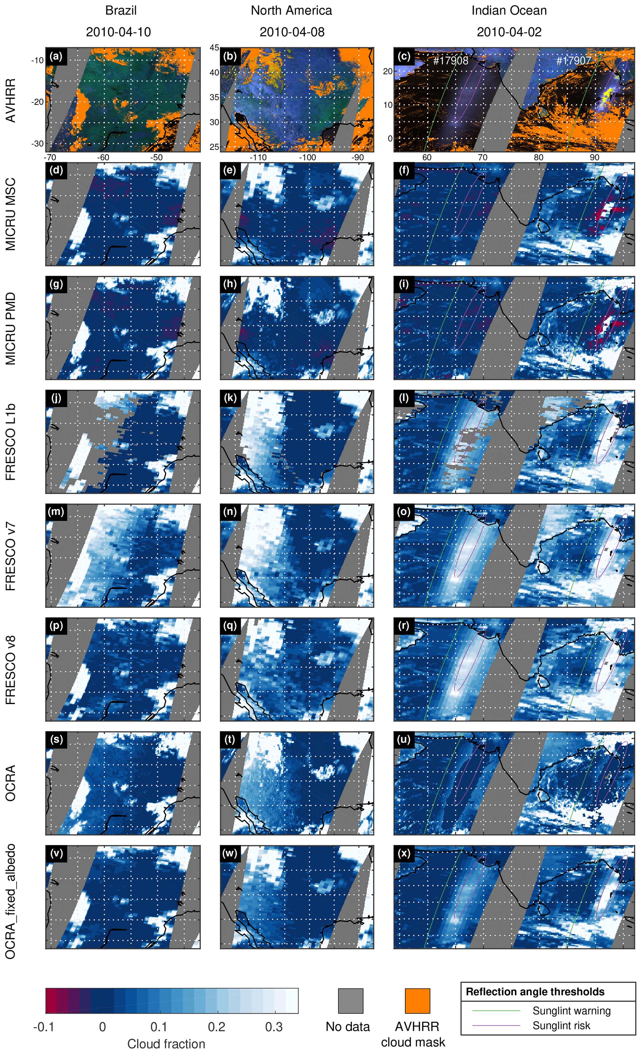
Figure 13Detailed comparison between different cloud fraction products over cloud-free scenes over land and ocean: Brazil on 10 April 2010 (left column), North America on 8 April 2010 (second column), and the Indian Ocean on 2 April 2010. The rows display cloud information from different sensors/products (from top to bottom): AVHRR false colour RGB image indicating areas where at least one AVHRR cloud test is positive (orange), MICRU MSC at 440 nm, MICRU PMD-PP at 460 nm, three FRESCO versions, OCRA, and OCRA_fixed_albedo. The colour bar is defined to resolve cloud fractions particularly below 0.3 and negative values. Areas without data are indicated in gray. Images in the right column contain swath data of two orbits featuring different sun glitter scenarios due to different wind conditions (see text).
MICRU MSC and PMD results show no significant cloud cover where also AVHRR does not detect clouds. Purple colours at the swath edges, however, indicate biased low CF results (Fig. 13d–i in cloud-free observations over both land and ocean. Over land, the MICRU results are consistent with the AVHRR cloud mask; e.g. CF contributions of singular clouds smaller than the GOME-2 pixel sizes are reproduced in Fig. 13e and h over North America. The bias of cloud-free observations is small and the colour bar range almost does not resolve the scatter around zero CF.
In the case of sunglint, the situation is more complex. In Fig. 13f and i, MICRU measurements scatter significantly as indicated within the area flagged with a sunglint warning (green edges). The scatter is only significant in the eastern swath (orbit 17907), whereas the western swath (orbit 17908) shows almost no scatter. The analysis of the wind fields (not plotted) reveals that wind speeds vary between 0 and 5 m s−1 for the cloud-free region of the eastern swath and between 3 and 4 m s−1 in the western swath, respectively. The interpolation of the wind fields is apparently not accurate enough for the eastern swath. The interpolation is limited by a spatial resolution of 1∘ and a temporal resolution of 6 h. Hence, MICRU CFs may be over- and underestimated in the event of heterogeneous wind situations and especially for very low winds. We conclude, however, that MICRU is able to model moderate Rmin contributions by sun glitter. When sun glitter is large (in the event of low winds), as indicated by yellow colours in the false colour background image of Fig. 13c, this correction is less reliable. Therefore, measurements flagged with a sunglint warning are screened from the statistical comparison studies below.
Figure 13 furthermore compares MICRU results to FRESCO and OCRA. Over land, the CF maps of FRESCO L1b and v7 measurements (Fig. 13j, k, m, and n) reveal significant positive biases in the western part of the swath. Cloud fractions larger than 20 % are detected even though AVHRR and MICRU both detect no clouds. FRESCO v8 displays a significant improvement over Brazil (Fig. 13p), whereas CFs over North America in Fig. 13q are still significantly biased in the west of the swath. Over eastern India (orbit no. 17907), however, all FRESCO versions are significantly biased high (Fig. 13l, o, and r). Switching to OCRA, Fig. 13s reveals significantly smaller positive biases of OCRA over Brazil compared to FRESCO L1b and v7. Over North America (Fig. 13t), however, a positive bias and scatter are significant. The biases of OCRA_fixed_albedo at MSC resolution are significantly smaller, especially over Brazil (Fig. 13v). Similarly, Fig. 13x shows significantly smaller biases over eastern India compared to the native OCRA results at PMD resolution in Fig. 13u.
Over ocean (right column in Fig. 13), biases in regions possibly affected by sun glitter are obvious in the FRESCO and OCRA data. FRESCO products are not correcting for this interference, leading to systematic positive biases because the increased intensity is apparently interpreted as reflecting clouds (Fig. 13l, o, and r). In contrast to FRESCO, OCRA corrects for the sunglint effect in the centre of the affected region (Fig. 13u), but interferences still persist for θr < 36∘, which is flagged by MICRU as sunglint warning.
3.3 MICRU
3.3.1 Global average cloud fraction
Figure 14 shows a global map of the average MICRU cloud fraction of 6 consecutive years using GOME-2A measurements. Therefore, it is a snapshot of the average CF at 09:30 LST. The averaging period starts in July 2007 and ends in June 2013. The map clearly reveals a statistically increased CF at the Intertropical Convergence Zone (ITCZ), off the western coasts of continents in the subtropics, and in the subpolar oceans. The comparatively high average CF over China indicates a significant bias due to aerosol scattering. Similar plots for MICRU PMD, FRESCO and OCRA are described in Appendix F.

3.3.2 MSC intercomparison
Figure 15 shows correlation density plots and bi-variate fits (Cantrell, 2008) of MICRU CF for channels 2, 12, and 14 with respect to MICRU channel 8 (see Table 1).
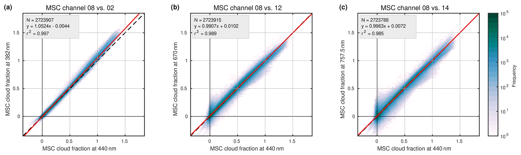
Figure 15Comparison between MICRU MSC channel 8 at 440 nm and MSC channels (a) 2 at 382 nm, (b) 12 at 670 nm, and (c) 14 at 757.5 nm for April 2010. The plots correspond to the combinations indicated by circles in Fig. E1a.
The comparison between MICRU evaluations at 382 and 440 nm shows an almost perfect correlation of r2 = 0.997 in Fig. 15a. The slope reveals a minute positive bias. Figure 15b and c reveal significantly increased scatter for comparisons with longer wavelengths, which is dominated by increased heterogeneities of the land surface reflectance because the scatter is almost independent of wavelength over ocean (not shown). It is important to note that in Fig. 15b and c the scatter in the y direction for small is larger than the scatter in the x direction for small . This indicates that the accuracy of CF is decreasing towards larger wavelengths.
Figure 15 furthermore indicates that the CF slope differs between MICRU channels, which is discussed in Sect. 4.1. Appendix E comprehensively compares results from MICRU channels and other cloud products.
3.3.3 MSC vs. PMD
Figure 16 shows CF comparison plots of two corresponding MSC/PMD evaluations. A spatial aliasing of m=0 is chosen for the comparison at 382 nm in Fig. 16a and m=1 at 519 nm in Fig. 16b, respectively. According to Fig. 3, these are the optimal choices of m, which is confirmed by the circled values in Fig. E2a, indicating a significantly higher correlation between MSC and PMD channels compared to the results neighbouring to the left and right.

Figure 16Comparison between MICRU MSC and MICRU PMD cloud fractions for April 2010: (a) at 382 nm and (b) at 519 nm. The plots correspond to the combinations indicated by circles in Fig. E2a.
Furthermore, the matrix results in Figs. E1b and E2a can be used to compare the influence of spatial vs. spectral aliasing. Due to the different readout scheme (Fig. 3), both cannot be perfectly fulfilled simultaneously, either spectral or the spatial alignment between MSC and PMD can be achieved. In Fig. E1b, the standard deviation of MSC measurements at 382 nm is slightly smaller (0.008) than for those at 424.5 nm (0.009). At 519 nm, however, the MSC values at 516.7 nm feature a smaller standard deviation (0.008) compared to those at 521.8 nm (0.009). Hence, spectral alignment seems favourable for PMD channel 1 at 382 nm, whereas spatial alignment seems favourable for PMD channel 4 at 519 nm. The linear coefficients of correlation in Fig. E2a, however, indicate that PMD channel 1 correlates slightly better to MSC channel 5 (0.998) compared to MSC channel 2 (0.997). Hence, spatial alignment is favourable if r2 should be optimal. For PMD channel 4, the deviation of the respective r2 values is < 0.001 (both 0.998). It shall be noted here that Fig. E2a also illustrates the importance for the correct choice of m. The correlation of PMD-PP at 519 nm with itself is significantly reduced from 1 to 0.994 if the value of m deviates by ±1.
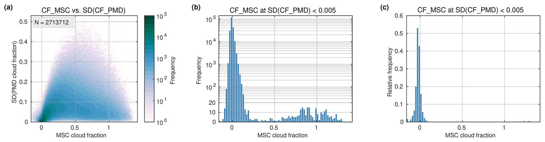
Figure 17Standard deviation (SD) of PMD cloud fractions within one collocated MSC pixel recorded in April 2010. PMD cloud fractions are obtained from PMD-PP channel 10 (m=1) with minimal spatial aliasing to MSC channel 10, which are both centred at 516.7 nm. (a) Density of PMD standard deviation and MSC cloud fraction; (b) histogram of MSC cloud fraction for a standard deviation of the collocated PMD measurements < 0.005 that is the lowermost row in panel (a); (c) relative frequency corresponding to panel (b). Note that the lower part of panel (b) is in linear scale; the upper part is in logarithmic scale.
The coefficient of correlation between MSC channel 10 and PMD channel 4 (m=1) of r2=0.998 is optimal for allowing a direct comparison and the investigation of the accuracy of small cloud fractions in the MSC product assuming that zero CF is physically only possible if all including PMD CFs are also zero. Therefore, standard deviations of PMD CFs within each MSC pixel are computed. Figure 17 shows the density of CF standard deviations vs. MSC cloud fractions. The maximum standard deviation is minimal for small and large CFs and maximal for a CF of approximately 0.5. The absolute and relative distributions of MSC measurements corresponding to a standard deviation of PMD CF < 0.005 are plotted in Fig. 17b and c, respectively. The width of the histogram bins is 0.02 CFs. Figure 17b peaks at −0.01 CFs and Fig. 17c at −0.03 CFs, which can be interpreted as an estimate for the accuracy of small MICRU CFs.
3.4 Comparison to other CF algorithms
3.4.1 MICRU vs. OCRA
Figure 13s and t in Sect. 3.2 suggest that OCRA measurements may be biased high in the western part of single cloud-free swaths over land. This observation is now investigated further based on monthly statistics. Figure 18a and b compare MICRU and OCRA measurements recorded over land and ocean, respectively. Most apparently, the slope of 1.35 indicates different definitions of the upper threshold. Figure E2c consistently confirms that OCRA overestimates large CFs compared to FRESCO and MICRU CFs. This is probably due to OCRA applying a scattering cloud model to define the upper threshold, whereas FRESCO and MICRU apply a reflecting cloud model. It needs to be noted that this comparison between OCRA and MICRU applies cropped data as described in Sect. 2.6, which may furthermore affect the overall slope. And indeed, the comparisons between MICRU MSC and OCRA_fixed_albedo in Fig. 19 result in more moderate slopes of 0.9 and 0.86 for land and ocean, respectively. Also the linear coefficient of correlation is slightly higher compared to the uncorrected OCRA values in Fig. 18.
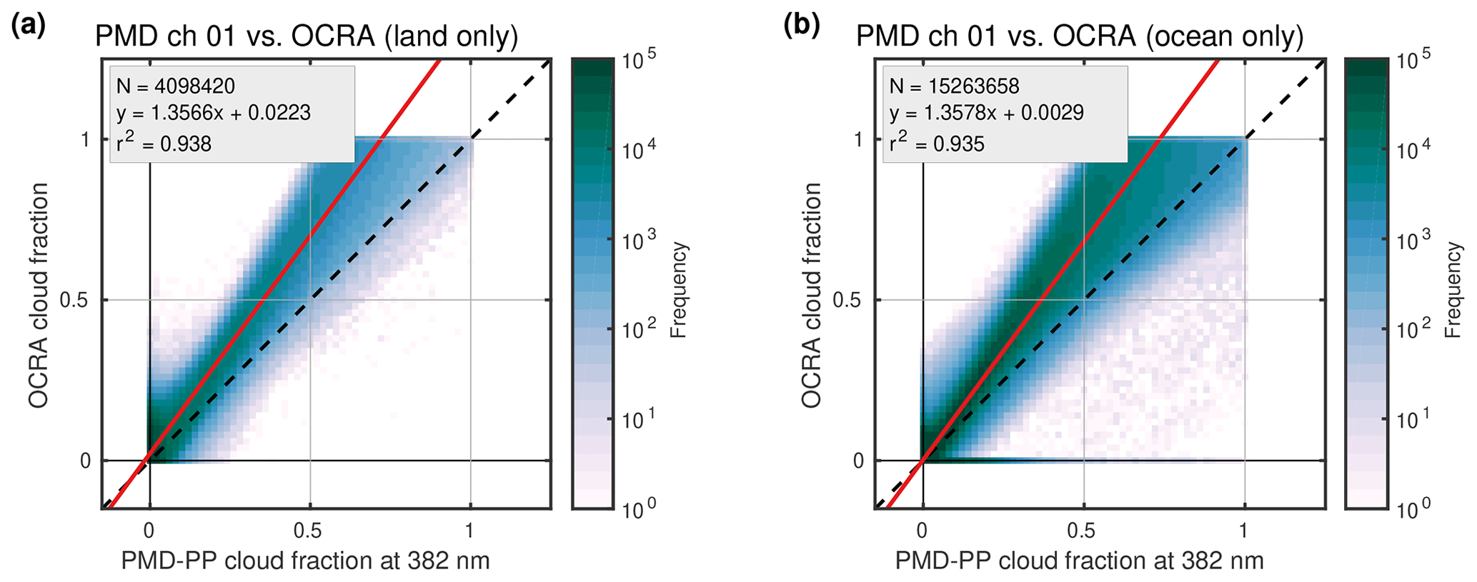
Figure 18Comparison between MICRU PMD at 382 nm and OCRA based on CF data from April 2010: measurements over (a) land and (b) ocean. This comparison applies cropped data.

Figure 19Comparison between MICRU MSC at 382 nm and OCRA_fixed_albedo based on CF data from April 2010: measurements over (a) land and (b) ocean. This comparison applies cropped data.
Secondly, it is focused on the scatter of very small cloud fractions. Figure 18 clearly shows that OCRA CFs for very small MICRU CFs scatter more than MICRU CFs for very small OCRA CFs (cf. Fig. E1b). Figure 18a and b investigate this feature depending on surface type land and ocean, respectively. Small OCRA CFs over land scatter significantly more for small MICRU CFs when compared to measurements over ocean. The same but less pronounced behaviour may be observed for OCRA_fixed_albedo in Fig. 19.
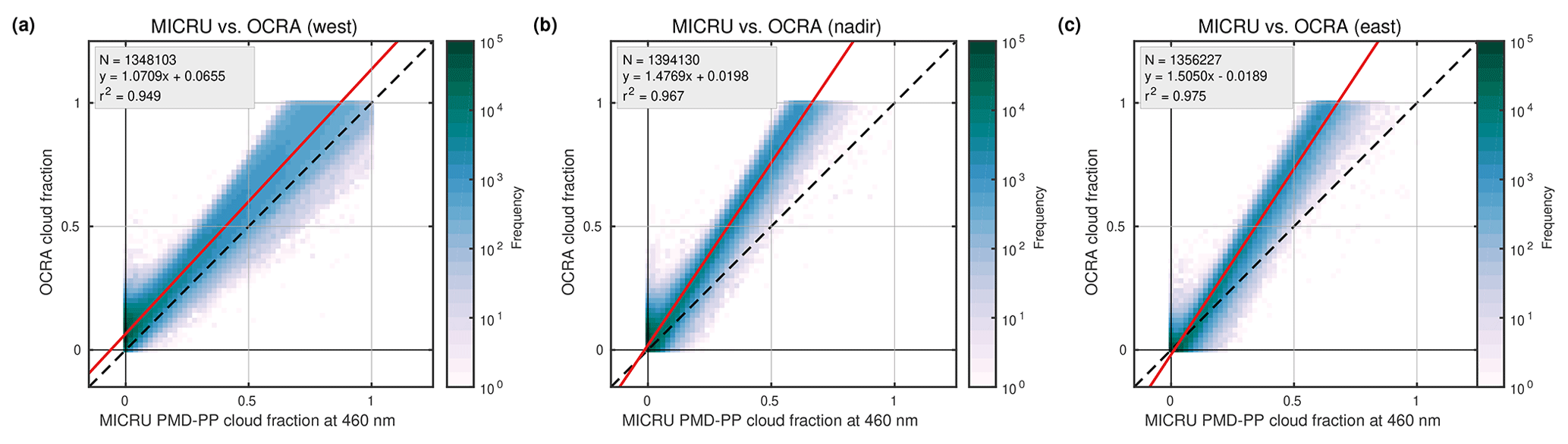
Figure 20Same data as Fig. 18a but for different viewing angles: (a) west, (b) nadir, and (c) east. This comparison applies cropped data.
Figure 20 shows a detailed comparison between OCRA and MICRU over land where the data are sorted according to the west, nadir, and east viewing directions, respectively. Focusing again on small CFs, a significant bias of 0.066 may be detected when averaging over the eight westernmost GOME-2 pixels of the swath (Fig. 20a), whereas the bias towards nadir and east is negligible (0.02). Furthermore, the scatter of small OCRA CFs is larger towards western compared to eastern viewing directions.
An additional view of the VZA dependence of MICRU and OCRA CFs is provided in Figs. 11a–c and 12a–c for land and ocean surfaces, respectively. Over land, the accumulation points of small OCRA MSC are significantly biased high for all negative VZA. The albedo correction for OCRA_fixed_albedo (Fig. 11c) improves the situation significantly, confining the accumulation point to CF < 0.1, which is still significantly larger than the MICRU CFs in Fig. 11a. Over ocean, both investigated versions of OCRA reveal a significant bias from sun glitter for positive VZA in Fig. 11b and c. Towards the west (negative VZA), the lower accumulation point of OCRA_fixed_albedo is more populated than MICRU.
3.4.2 MICRU vs. FRESCO
Figure 21 compiles the comparison between MICRU CFs at 440 nm and three FRESCO versions depending on surface type land or ocean, respectively. Overall, all FRESCO versions reveal a significantly higher scatter of small CFs compared to MICRU, which is similar to the comparison to OCRA. Furthermore, the scatter over land is consistently larger compared that to over ocean due to the increased albedo effect at 757 nm applied by FRESCO. The slope of the comparisons is close to unity due to a similar definition of the upper threshold. But there are specific differences between the FRESCO versions.
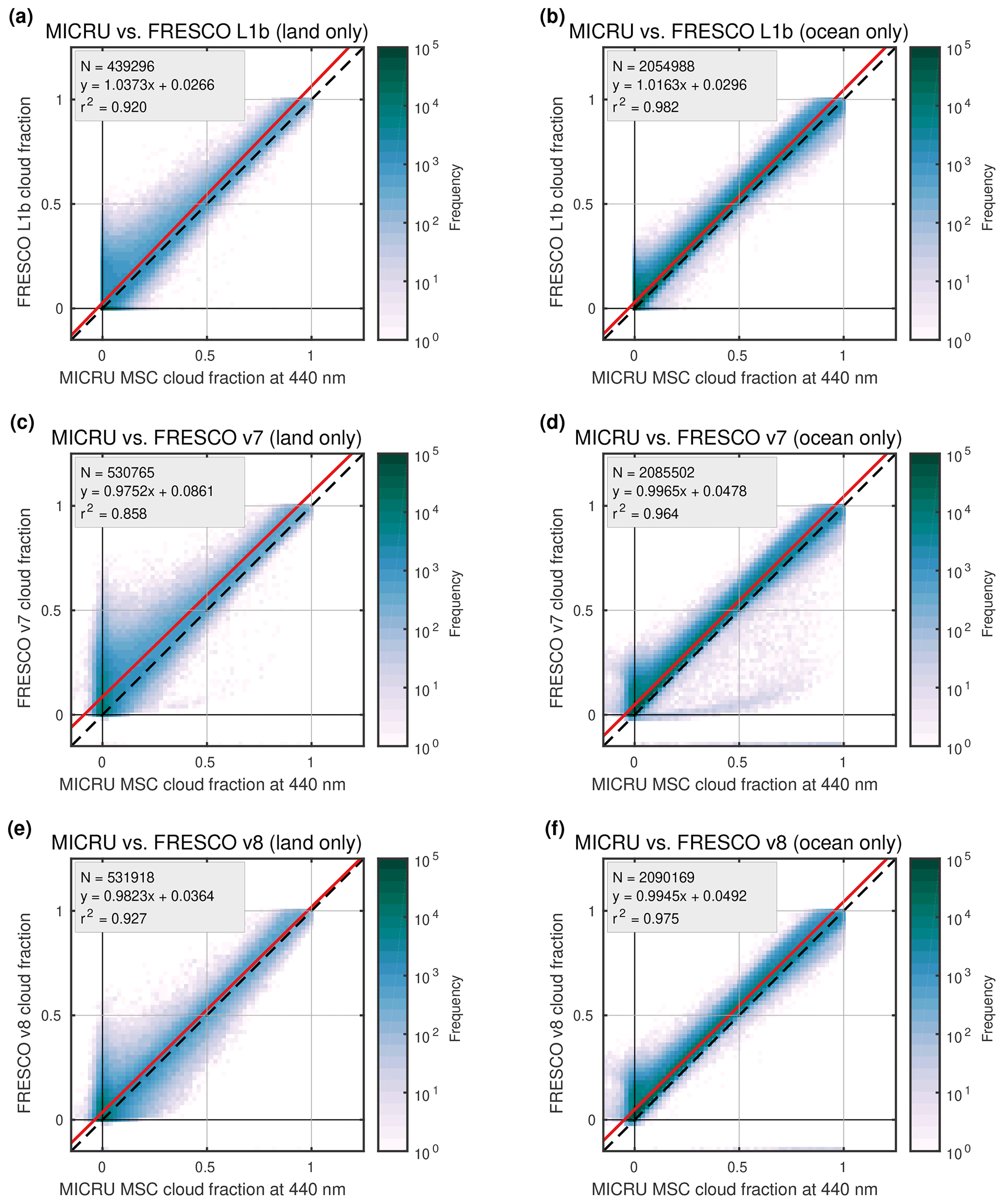
Figure 21Comparison between MICRU MSC at 440 nm and three different FRESCO versions based on CF data from April 2010: measurements over land (a, c, e) and ocean (b, d, f); FRESCO L1b (a, b), FRESCO v7 (c, d), and FRESCO v8 (e, f). The comparison to FRESCO L1b applies cropped data. The comparisons in panels (c)–(f) only exclude CF > 1.
The comparisons to FRESCO L1b in Fig. 21a and b feature smaller biases for small CFs than FRESCO v7 and v8, which is in agreement with Fig. E1b. The respective comparisons applying FRESCO v7 data in Fig. 21c and d reveal significantly larger scatter over both land and ocean. The bias over land is larger than 0.08, which seems to be a specific feature for FRESCO v7, as all other investigated products are less biased against each other (cf. Fig. E2b). The comparison over land in Fig. 21c includes FRESCO CFs up to 0.5 for MICRU CF equal to 0, which may be attributed to albedo effects along coasts as investigated below (Fig. 23). Figure 21d then shows a small quantity of unrealistic CFs smaller than 0.2 over ocean for MICRU CFs up to 0.8. Next, the comparison between FRESCO v8 and MICRU features a bias that is smaller compared to v7 but still larger than L1b. The scatter is significantly improved compared to v7, but the scatter of small FRESCO CFs for small MICRU CFs is still much larger than vice versa. In Fig. 21, it may be furthermore observed that both FRESCO versions (v7 and v8) feature CF < 0. This is an improvement considering that physical measurements are affected by noise.

Figure 22Viewing angle dependence of the comparison between MICRU at 440 nm and three different FRESCO versions over land. Same data as Fig. 21a, c, and e, respectively.

Figure 23Comparison between average cloud fractions from different algorithms: (a) MICRU PMD channel 8 at 440 nm; (b, d, f) FRESCO L1b, v7, and v8, respectively; (c, e, g) respective differences between MICRU and FRESCO. Averages include all nadir measurements ( 23.5∘, same as in Fig. 22b, e, and h, respectively) recorded in January, April, July, and October 2010. The T in panels (e) and (g) marks the location of Torreón municipality in Comarca Lagunera, Mexico (see text).
Similar to the comparison to OCRA, the comparisons between FRESCO and MICRU over land are now investigated depending on viewing geometry. Figure 22 consistently demonstrates that the western parts of the swath are biased due to BRDF effects. Largest biases are observed towards the west for FRESCO L1b and v7 (Fig. 22a and d), whereas the comparisons between FRESCO v8 and MICRU are almost independent of the viewing direction (Fig. 22g–i). It is furthermore noted that the comparisons between MICRU and FRESCO L1b for nadir and eastern viewing geometries in Fig. 22b and c reveal an almost identical scatter of small MICRU CFs for small FRESCO CFs and vice versa. This feature, however, is not visible in the comparison with the two more recent FRESCO versions, for which a significant number of small CFs are systematically biased (Fig. 22e, f, h, and i).
Figures 11d–f and 12d–f detail the VZA dependence of the three FRESCO versions over land and ocean, respectively. Over land, the accumulation points of small CFs are significantly biased high for negative VZA, especially for FRESCO L1b and v7. The distribution of FRESCO v8 CFs (Fig. 11f), however, is almost independent of VZA. Over ocean, the differences between the FRESCO versions are small and the bias from sun glitter is again significant, which is consistent with other results.
A final comparison between MICRU and FRESCO focuses on spatial features in average CF maps. Figure 23 compares average MICRU CF maps derived at 440 nm with three corresponding average maps from FRESCO data. The maps zoom on Mexico and its Pacific coast where interferences due to the land–sea contrast can be expected. All maps are computed using the same selection of data: January, April, July, and October 2010. In order to reduce potential interferences from BRDF effects (see Fig. 22), only the central third (nadir) of the swath is considered where 23.5∘. Significant differences between the four CF products are visible in the mean CF maps in the left column of Fig. 23 even though major features are similar. The difference plots in the right column quantify the differences. Comparing MICRU to FRESCO L1b in Fig. 23c reveals relatively high spatial gradients, especially at the coast of the peninsula. Furthermore, MICRU seems to be biased low in comparison to FRESCO L1b over the Pacific and mainland Mexico, especially in the north-east of the zoom image. The comparison to FRESCO v7 in Fig. 23e differs significantly. Here, FRESCO v7 is biased high throughout the image. Furthermore, FRESCO v7 CFs are biased low by more than 15 % along the coasts, which may be attributed to the low resolution sampling applied in the LER computation for this FRESCO version in combination with the larger albedo contrast between land and ocean in the wavelength range applied by FRESCO. For FRESCO v8 (Fig. 23g), this issue is partially reduced by applying LER maps with an increased resolution along coasts. Another feature in the comparison to FRESCO v7 and v8 in Fig. 23e and g is pointed out. Both average FRESCO data are biased high with respect to MICRU in central Mexico east of Torreón municipality, where the surface albedo is significantly higher compared to the surroundings. Hence, this feature may again be due to the comparatively low spatial sampling of the background LER maps and the red wavelength range, where the influence of the albedo on CF is larger compared to shorter wavelengths. In contrast, this interference is not visible in Fig. 23c where a MERIS background map sampled at higher spatial resolution is applied.
3.4.3 Temporal evolution and degradation
So far, the statistical evaluations are carried out on monthly data aggregates. Now, the temporal evolution of the different CF products is investigated with respect to small CFs. Here, the temporal evolution is studied based on the 15th percentile of monthly CF measurements framed by the 55∘ parallels. Preceding tests showed that 10 % to 15 % of GOME-2 MSC measurements are effectively cloud-free. The selection of the 15th percentile showed optimal contrast for this study and avoids saturation or normalisation effects. Figure 24 compiles the temporal evolution of selected CF products and groups them in order to highlight different comparative aspects.
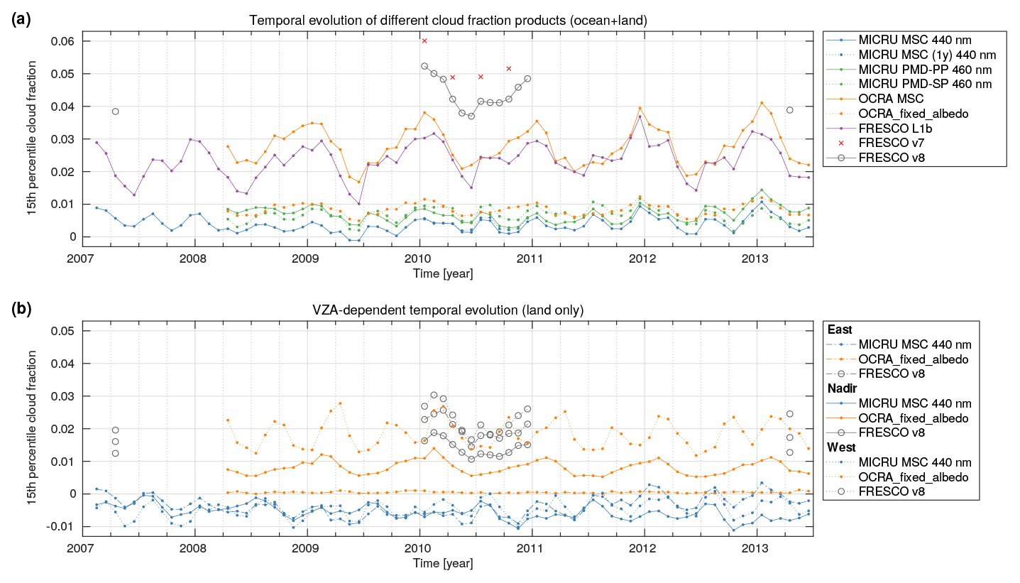
Figure 24Temporal evolution of the 15th percentile of monthly cloud fraction distributions: (a) comparison between selected MICRU channels, two OCRA versions, and three FRESCO versions, and (b) viewing angle dependency of MICRU, OCRA_fixed_albedo, and FRESCO v8. Note that the offset between the blue line in panel (a) and the average of the blue lines in panel (b) is due to a different data subset that is all vs. land only, respectively. FRESCO L1b and v7 results are omitted in panel (b) for the sake of clarity.
There are, however, no significant trends visible in the investigated time period.
Figure 24a compares the time series of different cloud products: MICRU MSC channel 8, the same MSC channel but applying only 1 year of data (dashed blue), the two MICRU PMD channels at a similar wavelength of 460 nm (Table 2), OCRA MSC, OCRA_fixed_albedo, and the three FRESCO versions. First off, the two MICRU MSC versions align almost perfectly. Apparently, reducing the time interval used to derive the LT parameterisation has an almost negligible effect in this comparison. Furthermore, the statistics of MICRU MSC, MICRU PMD, and OCRA_fixed_albedo data are almost identical, with the MICRU PMD and OCRA_fixed_albedo results being positively biased of ≈ 0.005. The amplitude of bi-annual variations is of the same order for the MICRU versions and less pronounced for OCRA_fixed_albedo. In contrast to the MICRU results, OCRA and FRESCO results feature a larger amplitude of at least 0.01 and an increased annual instead of bi-annual oscillation. For all products, the overall trends are negligible compared to the annual variations.
Figure 24b details the CF statistics depending on VZA over land (see Figs. 20 and 22). The plot confirms the aforementioned results: MICRU shows negligible VZA dependence of the 15th percentile. For FRESCO v8, the 15th percentile of nadir measurements (solid gray line) is approximately 0.01 smaller compared to measurements in the eastern and western thirds of the swath. The VZA dependence in the OCRA_fixed_albedo percentiles is significantly larger compared to MICRU and FRESCO. OCRA data reveal a clear east-to-west trend, while FRESCO v8 features minimal CF values in the centre third of the swath. The CFs in the western third of the swath of OCRA_fixed_albedo (dotted orange line) average to 0.02, while the average is close to zero in the eastern third of the swath.
4.1 MICRU
Figures 8 and 9 illustrate the Tmin retrieval at two different sites and wavelengths. The residuals in both examples (Figs. 8f and 9f) are on average significantly smaller than the targeted 0.04 accuracy. Systematic contributions from degradation, seasonal variability, VZA dependence, and sun glitter are small. This indicates that Eq. (4) is sufficient to parameterise Tmin for GOME-2A. Figures 13 and 24b also support this conclusion. The periodic structures in the west of Fig. 8e, which are also visible but less pronounced in Fig. 9e, may be mostly attributed to the anisotropic reflectivity over land. Figure 11 suggests that this anisotropy may be underestimated by the operational CF products. In Fig. 8e, there seems to be an upward trend and a shift of the apex towards east over time. Both may be attributed to the degradation of this particular MICRU channel (cf. Fig. D1a and d). Furthermore, also local changes of land use, vegetation type, or precipitation climatology may lead to shifts in the lower threshold, which would be linearised by the applied Tmin model. These additional local trends may be reproduced by the MICRU algorithm as Fig. C1d and g illustrate.
Equation (4) models the residual VZA dependence. Figure 10 shows that the VZA dependence and its temporal dependence vary between GOME-2 channels even though they are measuring in the same wavelength region. This indicates that the instrumental contribution to the residual VZA dependence is at least of the same order as possible inaccuracies of RT used to invert the surface LER. Hence, this issue cannot be solved by a more accurate RT but needs to be corrected for empirically. Furthermore, degradation needs to be accounted for and it needs to be noted that the design of MICRU would allow degradation models different from Eqs. (4) and (10). For example, discrete functions and prescribed degradation are both possible to be included.
Considering the influence of surface BRDF effects on MICRU CFs, our results support the discussion by Lorente et al. (2018) that the LER model systematically underestimates the surface reflectance in forward direction corresponding to the eastern part of the GOME-2 swath. Figures C1f and D1c show that the average apex offset is biased high. The minimum gradient of the polynomial is more frequently in the eastern part of the swath. This suggests stronger contributions from the surface BRDF in the western part of the swath in accordance with Lorente et al. (2018). Therefore, MICRU CFs in Figs. 11, 12, 13, 20, and 22 are consistently smaller in the western part of the swath when compared to OCRA and the three FRESCO versions because OCRA and FRESCO both apply a constant surface reflectance model, whereas MICRU applies an empiric VZA dependence model. This effect is almost independent of wavelength and consistent for all MICRU channels (cf. Fig. 15 and Appendix E). It needs to be noted, however, that also OCRA applies an empirical VZA correction based on global monthly means (Lutz et al., 2016).
Lorente et al. (2018) furthermore claim that surface effects are stronger for longer wavelengths where atmospheric scattering is weaker. Figure D1b may support this claim: the average curvature of the residual VZA dependency decreases with wavelength but its variance increases. This observation is consistent for all three channels and suggests that, at shorter wavelengths, the residual VZA dependency is due to a combination of instrumental and RT effects, which are similar for the ensemble of measurements. At larger wavelengths, however, the surface introduces a larger variance due to stronger spatial and season heterogeneities. However, the wavelength dependency of the apex offset in Fig. D1c is ambiguous. The average apex offset peaks between 450 and 700 nm for two out of three GOME-2 channels. The variance, on the other hand, is minimal for shorter wavelengths. Therefore, retrieving CFs in the UV–blue spectral range is in any case beneficial in order to reduce interferences with surface albedo and type.
In addition to interferences with BRDF effects, there is another drawback of retrieving CFs at larger wavelengths (Sect. 3.3.2), which is caused by the spectral surface albedo and its heterogeneity increasing with wavelength. CFs retrieved at 382 and 440 nm correlate better compared to those retrieved at the O2-B and O2-A bands at 670 and 757.5 nm, respectively. This effect is studied more systematically in Fig. E1b, revealing a significant increase of the standard deviation of small CFs between 521.8 and 670 nm. The average CF maps (Figs. F1, 14, F2, and F3) of MICRU CFs at 382, 440, 670, and 757.5 nm, respectively, reveal significant systematic biases of the bright tropic deserts at 670 and 757.5 nm, notably aver Africa and Australia. At 382 and 440 nm, the MICRU results over bright desert areas are significantly smaller than all other results and may therefore be assumed more reliable. This assumption is confirmed in Fig. 13, where MICRU CF results over North America and eastern India, which are significantly brighter compared to Brazil, are not significantly biased. These maps furthermore indicate systematic CF biases from anthropogenic aerosols over East Asia and residual clouds in the tropics of South America and Africa.
Another aspect of the MICRU MSC channel intercomparison are differences at different wavelengths for high values of CF and hence slopes deviating from unity as, for example, shown in Fig. 15a. CFs at 382 nm are biased high with respect to those retrieved at 440 nm, while the intercept at zero CF is negligible. Hence, the definition of Tmax apparently deviates between MICRU channels, which should be independent of surface effects. Figure E2c comprehensively compares the slopes of all MICRU channels. There is a significantly biased slope for MSC channels 1–4 retrieved at 389.7 nm and below. This step between MSC channels 4 and 5 may be attributed to the application of different GOME-2 bands, specifically bands 2B and 3, from which the MICRU channels are extracted (Table 1). Hence, we conclude that differences between MICRU channels at high CF values are dominated by instrumental effects and calibration deficiencies of the input data. We would like to note that we observed also the CF accuracy degrading near GOME-2 band edges when fine tuning the MSC channel definitions (Table 1). The degradation depends only weakly on kernel width, leading to the conclusion that this is a broadband effect. Furthermore, interferences with molecular absorption and atmospheric scattering above the clouds resulting in a wavelength dependent R may also cause a systematic slope bias. It needs to be noted, however, that the influence of the slope on the accuracy on small cloud fractions is minor.
From the systematic studies compiled in Figs. E1 and E2c, we may conclude that MSC channels between 424.5 and 521.8 nm are most consistent. The varying slope in band 2B may be influenced by instrumental effects. For cloud height retrievals using the O2-A band, MICRU channels 4 and 7 centred at 389.68 ad 433.4 nm, respectively, may be a good option for GOME-2 as they offer reasonable spatial aliasing (Fig. 3). There is a slight priority for channel 7 when considering the mean and standard deviation of small CFs in Fig. E1a and b.
The comparison between MSC and PMD channel results with minimal spatial alignment in Fig. 16 shows an almost perfect correlation and biases ≤ 0.4. The correlation in the UV is slightly lower compared to the visible, which may be caused by the inferior spatial aliasing in the UV. The comparisons between MSC and PMD furthermore reveal a slope significantly smaller than 1. Figure E2b reveals that this is a minor feature and may be explained by calibration differences between the different GOME-2 channels. However, the slope is dominated by differences of the definition of the UT, which are not accounted for by MICRU. This behaviour has a minor effect on the accuracy of the LT.
The comparison between MSC and PMD measurements allows us to estimate the influence of spatial (i.e. temporal) and the spectral alignment. Figure E2a confirms a maximum correlation for optimal m as expected. The influence of the spatial alignment parameter m is found significant and deviations by ±1 degrade the correlation from 0.998 to 0.992 for MSC at 516.7 nm. Results comparing spatial vs. spectral alignment are not very clear. At least for PMD channel 4 (PMD-PP centred at 519 nm), spatial alignment seems slightly favourable over spectral alignment, which would be perfect for MSC channel 11 (Fig. E1b).
Hence, MSC channel 10 is selected over channel 11 to be compared to PMD-PP channel 4 with m=1 in order to investigate the absolute accuracy of small CFs. The comparison between the standard deviation of PMD CFs within one MSC pixel in Fig. 17 indicates that the systematic bias of MICRU CFs is of the order of −0.03.
Figure 24 finally shows that small MICRU CFs have a negligible trend over the investigated period of more than 6 years. The variations of the 15th percentile are smaller than 0.01. Clearly, CFs at different viewing directions are significantly more consistent for MICRU compared to OCRA and FRESCO.
4.2 OCRA
OCRA CFs are compared to MICRU results based on singular orbits and exemplary monthly statistics. Both approaches consistently reveal that OCRA CFs are biased high for observations towards the west (Figs. 13s, t, and 20a). This indicates that BRDF effects have a stronger influence on OCRA results for observation geometries opposing the Sun and that the empirical VZA correction performed by OCRA is not sufficient. OCRA_fixed_albedo results, however, indicate that considering the cloud albedo by ROCINN significantly lowers the biases between MICRU and OCRA/ROCINN CFs (Figs. 13v–x, 19). OCRA_fixed_albedo CF values in the eastern third of the GOME-2 swath have similar statistics to MICRU (Fig. 24b). It needs to be noted, however, that comparisons to OCRA_fixed_albedo may only be performed at MSC resolution because the required ROCINN cloud albedo values are not available in PMD resolution. Therefore, all comparisons to OCRA at PMD resolution are affected by a different cloud albedo.
Considering the bias of small MICRU CFs of −0.03, the bias of OCRA measurement in the western third of the swath can be estimated to 0.095 on average over land. These biases may be even larger depending on observation geometry and surface type (Fig. 13t).
The overall statistics in Fig. 18 indicate that small OCRA CFs are on average less biased when taking into account the negative systematic bias of MICRU (Sect. 3.3.3). The accuracy of singular OCRA measurements, however, is significantly and consistently lower compared to MICRU, as revealed by the larger scatter of OCRA CFs for very small MICRU CFs than vice versa (Figs. 18, 20, and E1b). Again, the application of OCRA_fixed_albedo improves the comparison in Fig. 19 significantly compared to OCRA at PMD resolution (Fig. 18). The remaining excess scatter of small OCRA_fixed_albedo compared to small MICRU CFs may be explained by the spatial aliasing effect intrinsically affecting all OCRA evaluations, which combine PMD measurements from three PMD bands with slightly different acquisition times.
From the investigation of OCRA CFs over ocean in Fig. 13u, it can be concluded that OCRA's empirical correction algorithm is a bit too optimistic. While large contributions by sun glitter seem to be removed, the area at larger θr are still positively biased. In regions of very strong sun glitter (yellow areas in Fig. 13c), OCRA seems to properly account for this effect on PMD resolution. OCRA_fixed_albedo, however, is again affected by sun glitter as indicated in Fig. 13x. It is noted that the conservative MICRU sunglint warning flag contains the affected regions and that also OCRA contains a sunglint flag.
4.3 FRESCO
Three different versions of FRESCO CFs are compared to MICRU MSC results based on singular orbits, exemplary monthly statistics, and average nadir maps. The different approaches for the background maps of the FRESCO versions are clearly visible in Figs. 22 and 23. Small FRESCO CFs over land are significantly biased high for western observation geometries by 0.17 and 0.21 on average for FRESCO L1b and v7, respectively. In contrast, the comparison between FRESCO v8 and MICRU is almost independent of the VZA. Therefore, we conclude that the consideration of BRDF effects in FRESCO v8 displays a significant improvement compared to preceding versions of the product.
On the other hand, however, Fig. 23 shows that interferences with the coast are minimal for FRESCO L1b, whereas both newer FRESCO versions are significantly biased high at coasts and inland. This issue is slightly improved in FRESCO v8, where GOME-2 background LER data are sampled at a 4 times higher resolution at coasts. This specific positive bias along coasts may interfere with the processing and evaluation of tropospheric trace-gas products from GOME-2 applying FRESCO because it leads to filtering a significant amount of measurements there when a CF-threshold filter is applied. Assuming a significant fraction of the world's population resides along coasts, this interference is considered significant. Less coastal measurements would be applied using FRESCO L1b, but this would come with the cost of filtering many measurements in the western part of the swath, as investigated in Fig. 22.
Compared to MICRU, FRESCO results are biased high, as indicated in the top right panel of Fig. E1a. The mean biases of FRESCO v7 and v8 are between 0.05 and 0.07, which is unrealistic even when considering the systematic bias of MICRU CFs. In this light, FRESCO L1b CFs, however, are probably less biased on average compared to MICRU.
The scatter of FRESCO CFs for very small MICRU CFs, however, is consistently larger for all FRESCO versions than vice versa. This may be attributed to the application of radiances close to the O2-A band as discussed above. From the comparison of MICRU CFs at different wavelengths, we may furthermore conclude that the attempt by Desmons et al. (2019) to apply FRESCO at the O2-B band may not fully mitigate significant interferences with heterogeneities of the absolute surface albedo.
In general, it appears that features in the comparison between one FRESCO version and MICRU do not appear in the comparison with the other FRESCO versions. We therefore conclude that MICRU reveals actually less systematic features than all three considered FRESCO versions.
MICRU is a cloud fraction retrieval algorithm based on satellite radiance measurements of backscattered solar radiation. The MICRU algorithm achieves an accuracy of 0.04 in calculating small effective CFs from spectroscopic satellite measurements. This is a prerequisite for accurate trace-gas retrievals because clouds in most cases determine the radiative transport within each satellite measurement. The unique feature of MICRU is the application of an empirical BRDF surface model accounting for viewing angle dependencies in the cloud retrieval. The paper demonstrates that MICRU CFs depend significantly less on VZA compared to other available CF products for GOME-2 and hence are significantly more accurate. MICRU determines the lower threshold from the measurements themselves, furthermore reducing biases due to calibration and degradation issues.
As a proof of concept, we applied MICRU to GOME-2A data, but the algorithm is also applicable to similar spectroscopic satellite missions like SCIAMACHY, OMI, S5P/TROPOMI, and Sentinel-5/UVNS. Furthermore, MICRU can also process UV–vis imager data like AVHRR, MERIS, MODIS, or Sentinel-2/MSI (multi-spectral instrument) due to its scalable design.
Our results confirm that MICRU is able to accurately retrieve small CFs over a wide spectral range, which renders it an optimal choice for tropospheric trace-gas retrievals. These should use a cloud product based on radiance measurements of similar wavelength and spatial sampling so that the correlations between cloud and trace-gas retrievals are optimised. For example, satellite instruments like Sentinel-5 have an inter-band offset of up to 30 %, which deteriorates the applicability of particularly small cloud fractions retrieved in the red spectra range (e.g. FRESCO) to differential optical absorption spectroscopy (DOAS) products like NO2 and HCHO retrieved in the UV–blue spectral region.
In conclusion, applying radiances recorded in the UV–blue spectral range is advantageous over the red spectral range in order to reduce surface effects. Furthermore, spatial alignment effects between MSC and PMD channels may be minimised by choosing appropriate spectral convolution kernels. In order to test the applicability of MICRU to data from recent satellite missions spanning less than 6 years, it was applied on a data set reduced to 1 year. Results of this alternative retrieval are found to provide sufficient accuracy. Hence, MICRU may be applied on satellite missions offering less data than the GOME-2A mission with confidence.
MICRU applies an iterative threshold technique to retrieve the lower accumulation point Tmin. The method is similar to the threshold method applied by HICRU (Grzegorski et al., 2006), where Rmin is assumed to only depend on time and viewing direction. For HICRU, this dependency could be resolved manually because the number of discrete VZAs was small, and therefore the lower accumulation point could be efficiently retrieved in an image processing manner. MICRU, however, assumes a more complex behaviour of Tmin and therefore incorporates a non-linear least-squares fit in every iteration of the lower accumulation point determination algorithm.
The basic idea behind iterative surface fitting is that the lower envelope of measurement set Ω (blue dots in exemplary Figs. 8b and 9b) is approximated by iteratively filtering measurement tuples fulfilling
where y(β) is the fit result and τ is a positive threshold. β denotes the result vector of Eq. (4):
The accuracy and the convergence of the method depend on the choice of τ (Grzegorski et al., 2006), the applicability of the Tmin model, the stability of the surface fit, and the initial values β0. Compared to HICRU, MICRU introduces two improvements: (1) an adaptive scaling of τ reducing the number of a priori assumptions, and (2) the application of a surface fit. The surface fit incorporates parameter constraints (Table 5), and therefore the trust-region-reflective algorithm (Coleman and Li, 1994, 1996) is applied.
The initialisation of the fit defines β0 and an initial selection vector V0. The selection vector Vi defines the subset of measurements , on which the (i+1)th iteration of the surface fit is applied. Table 5 provides initial values β0 except for a0, which is set to the median of LER(Ω). V0 is set true for all LER measurements fulfilling , where σ0 is the standard deviation of residual vector . The initial threshold τ0 is set to 0.012.
The ith iteration consists of the following steps: fit Eq. (4) to Ωi with initial guess βi−1 yielding βi. The residual vector is then , defining the measurement set used in the next iteration through
where σR is again the standard deviation of R. The second condition in Eq. (A3) filters outliers of the measurements distribution towards −∞.
After that, the threshold for the next iteration is determined. τi+1 depends on the retrieved mean LER; that is, the threshold becomes larger for brighter surfaces. The adjustment is retarded to steps of δτ=0.002. The upper limit τmax is defined. τmax increases linearly with : for and τmax = 0.1 for = 1. Then, τ is increased if
or decreased if
Iterations terminate if at least one of the following four conditions is true: number of iteration steps exceeds imax = 40, invariance of selection vector (Vi+1 = Vi), invariance of result vector (βi = βi−1), or Ωi+1 includes less than eight data points.
The result is β = βi, corresponding to a remaining set Ωi (red dots in Fig. 8b) defining Tmin as a function of , , θs, and rg in a specific geospatial bin. Diagnostic metrics for filtering (Sect. 2.5.3) are the number of elements in Ωi, its ratio to the number of elements in Ω0, and the number of iterations i.
The merging process consists of the following steps:
-
Extrapolate all results to highest resolution.
-
Discard result bins fulfilling
-
i < 4, or
-
a0 ≤ −0.5 for φ > 80∘ S.
-
-
Additionally, filter oceans bins where
-
120, or
-
1000 for and 65∘
is fulfilled, except in the coarsest resolution realised in binning no. 7.
-
-
Additionally, filter bins over land with .
-
Filtered maps are merged from coarse to fine resolution in order to maintain the highest resolution possible.
-
Empty bins – or gaps – are extrapolated as follows:
-
For φ≤ 80∘ S, zonal means are copied into the gaps; if there are no data at the same latitude at all, β from one row towards the north are applied.
-
Remote gaps, like islands or lakes, which are more than 6∘ longitude and 3∘ latitude away from a valid bin, are filled with zonal mean values.
-
Remaining gaps, e.g. at coasts, are filled by successive applying a Gaussian convolution kernel with a 1σ diameter of 3∘ longitude and 1∘ latitude.
-
-
Set ag = 0 for 65∘.
Figure C1 shows an exemplary stitching result for MSC channel 2. The spatial origin of the finally applied fit results is compiled in Fig. C1a: fit results from the highest resolution – binning no. 1 over land and binning no. 4 over the ocean – are in dark blue colour. Extrapolated bins are coloured in yellow. Coastlines typically apply coarser resolutions because of the poorer statistics and the 90 % cut-off criterion for the respective surface types. Polar oceans appear in light blue or orange colours because frequent clouds and bright sea ice significantly reduce N∗.
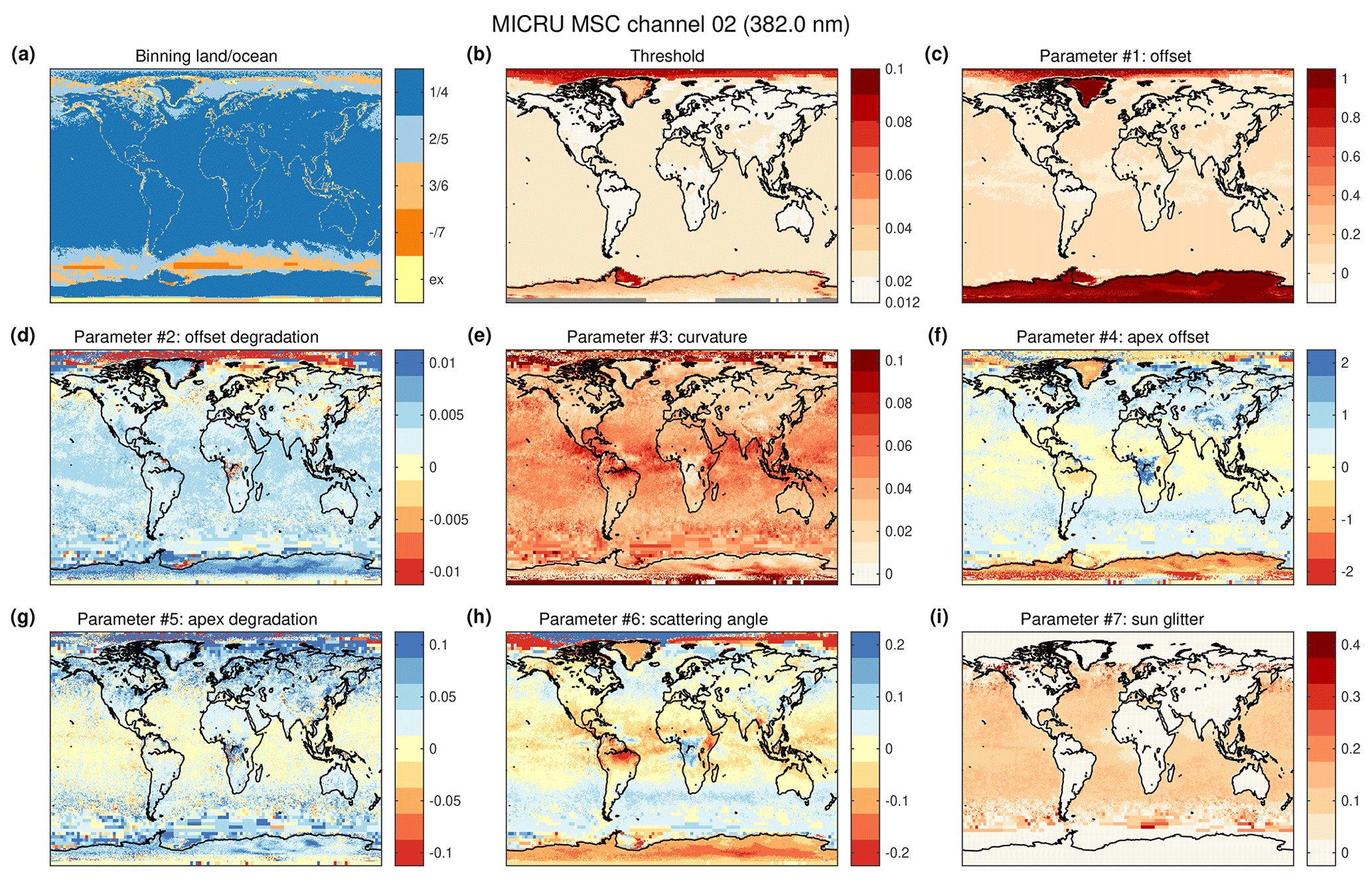
Figure C1Parameterisation of the lower threshold (LT) for MSC channel 2 after post-processing: (a) binning over land and ocean, (b) final threshold Tmin, (c) offset, (d) offset degradation, (e) curvature, (f) apex angle, (g) apex degradation, (h) scattering angle, and (i) sun glitter. In panel (a), colours other than dark blue indicate regions where the resolution is reduced or extrapolation (ex) is applied. Coast-containing pixels display land results.
Figure C1 is a merged Tmin map of all binned Tmin results for MSC channel 2. It is the base LUT for calculating Rmin globally. Figure C1b indicates that τ increases over water and desert regions with larger LER. Figure C1c–i illustrate the geographical dependence of the fitted surface parameters. A significant latitudinal dependence and interferences with the increased cloud probability at the ITCZ can be observed for all parameters. A significant land–sea contrast is visible for the apex degradation in Fig. C1g: the apex seems to shift systematically less over land. Furthermore, there is a significantly different behaviour of the apex angle and scattering angle dependence over the rainforest regions between South America and Africa in Fig. C1f and h, respectively. Both regions feature a comparatively large cloud probability and hence fewer statistics available for the Tmin retrieval.
It is noted that Fig. C1d and g reveal that both trend terms are latitudinally correlated with the opposite sign. A discussion of independent terms is therefore difficult. This observation, however, confirms an overall degradation of the VZA dependence as shown in Fig. 7.
Sunglint is not constant throughout Fig. C1i and therefore cannot be corrected for a priori. Specifically, panel (i) indicates lower values in the ocean west of equatorial Africa and India. Towards the poles, scatter increases as sunglint contribution diminishes. Over the Amazon, interestingly, there is a clear signal from sun glitter, which was not expected a priori, illustrating the gain by fitting this parameter also over land.
Figure D1 compiles the average wavelength dependency of the Tmin parameters for the MSC and PMD MICRU channels. Apparently, offset degradation is much more an issue for MSC and PMD-PP when compared to PMD-SP (Fig. D1a), which is in accordance with the findings from Fig. 10. The VZA dependence is consistently stronger in the UV compared to MICRU channels at longer wavelengths (Fig. D1b) but relatively smaller for PMD-PP as already discussed above. The wavelength dependence of the apex degradation in Fig. D1d seems to be much more complex, changing signs below 500 nm. The wavelength dependence of as is small compared to the overall variability in Fig. D1e. ag values in Fig. D1f are increasing with wavelength, suggesting Rayleigh scattering is damping the contribution from sun glitter in the UV.
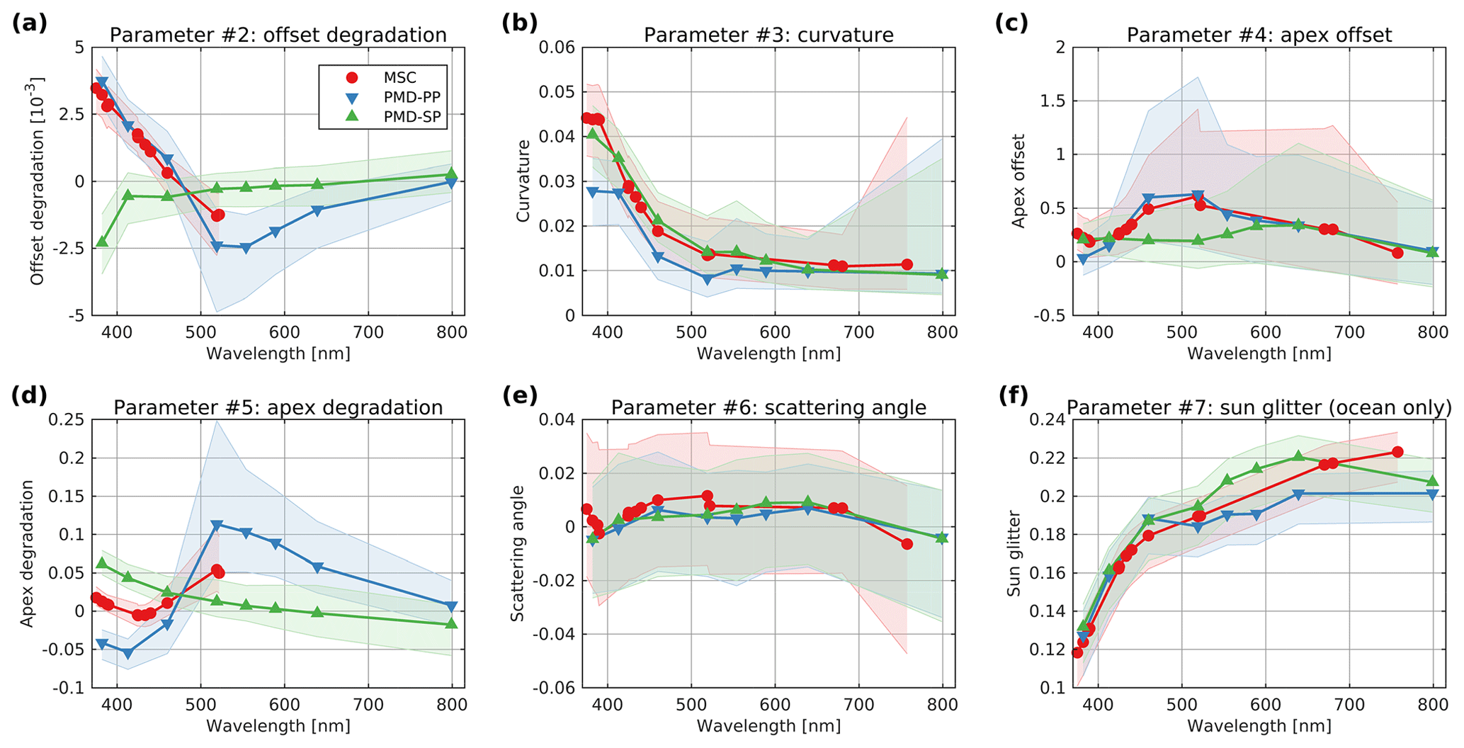
Figure D1Wavelength dependency of Tmin parameters: (a) offset degradation, (b) curvature, (c) apex offset, (d) apex degradation, (e) scattering angle, and (f) sun glitter. MSC channels are in red, PMD channels 1–8 in blue, and PMD channels 9–16 in green. Interconnected data points are median fit parameters. Transparent areas include 50 % of all results with boundaries at the 25th and 75th percentiles.
Figures E1 and E2 show a selection of comparisons between different MICRU MSC, MICRU PMD, FRESCO, and OCRA cloud products for April 2010. Figure E1a and b show the mean CF and standard deviation of selected CFs for the product in the x direction. The selection includes only those measurements fulfilling of the product in the y direction. As a reference, results in Fig. 15, which are the results where MICRU MSC channels 2, 12, and 14 are compared to MICRU MSC channel 8 evaluated at 440 nm, correspond to the results in the second row as indicated by circles in Fig. E1a.
Focusing on the inter-MSC comparison, the upper left block in Figs. E1 and E2, one observes that the MICRU results are relatively consistent for all MICRU channels. The standard deviation in Fig. E1b reveals a significant jump between 521.8 and 670 nm, which was already observed in Fig. 15. Figure E2a and b show that the correlation degrades and the deviation of small CF increases with increasing spectral distance. The slope, which is dominated by Rmax, reveals a significant jump between 389.7 and 425.5 nm in Fig. E2c, coinciding with a step from MSC band 2B to band 3 (Table 1).
MSC applying less data
In addition to the standard MSC evaluation integrating 6 years of measurements (Sect. 2.1.1), an evaluation using only 1 year of data is performed in order to simulate the performance of MICRU if applied to shorter data sets. We chose the year 2010 because it ranges approximately in the centre of the standard evaluation period where CF accuracy may be assumed optimal (see Sect. 3.4.3). For this special evaluation, the parameters accounting for degradation (at and aa1 in Table 5) are constrained to 0 for all MSC channels. The results of this simulation are included in the result matrices in Figs. E1 and E2 and denoted as “1 year”.
The circles in Fig. E1b indicate the entries, where the new results are compared to the standard results, which are located one column to the left. All circled values are larger compared to the standard evaluation. This indicates that small cloud fractions are less accurate if a shorter evaluation period is chosen. The corresponding matrix entries in Fig. E1a indicate that small cloud fractions retrieved at 382 nm are more deviated compared to the standard evaluation (−0.3) compared to those at longer wavelengths, where corresponding entries are negligible (denoted by ⋅).
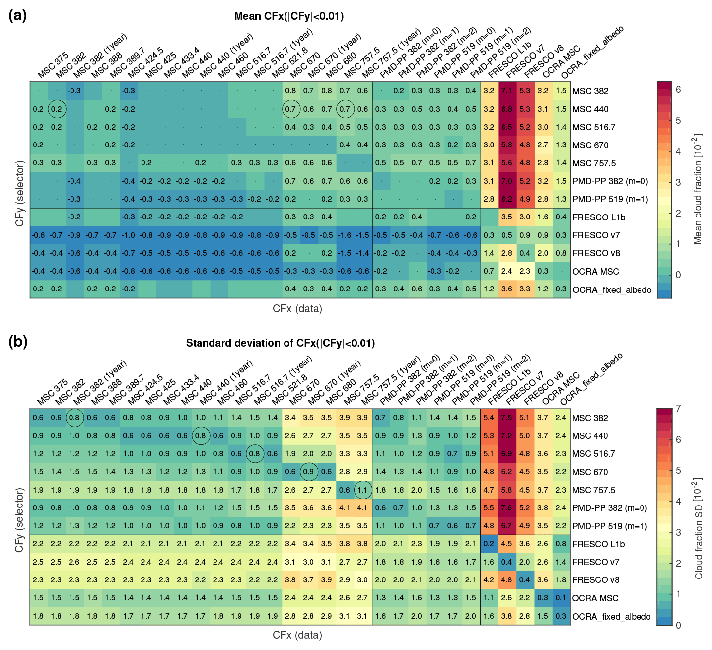
Figure E1Tabular intercomparison of MICRU and external cloud fraction results for April 2010: (a) mean CF of product listed in the x direction selected by corresponding product in the y direction with an absolute CF < 1 %; (b) same as panel (a) but listing the standard deviation. The circled values in panel (a) correspond to Fig. 15. The circled values in panel (b) indicate values comparing data of the same MICRU channel but different evaluations periods: 1 year vs. the standard data set applying 7+ years.
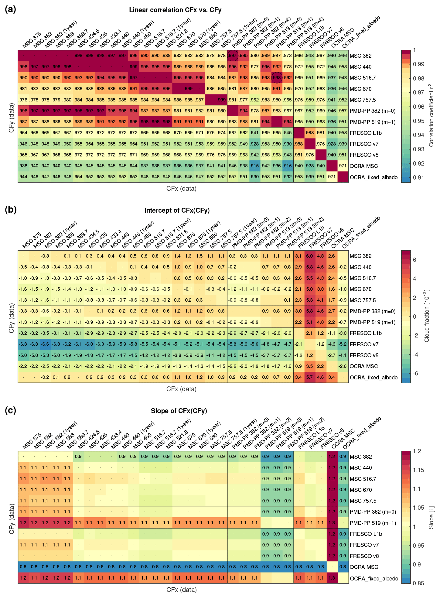
This section compiles global average cloud fraction maps of MICRU MSC channels 2, 12, and 14 (Figs. F1, F2, F3), FRESCO L1b (Fig. F4), FRESCO v7 (Fig. F5), FRESCO v8 (Fig. F6), MICRU PMD channel 4 (Fig. F8), OCRA (Fig. F9), and OCRA_fixed_albedo (Fig. F7) similar to Fig. 14 in Sect. 3.3.1, applying MICRU MSC channel 8 in the main body of the paper. MICRU MSC and FRESCO L1b maps are compiled from 6 years of data collected between July 2007 and June 2013. Averages of MICRU PMD and OCRA data begin 1 year later. FRESCO v7 data (Fig. F5) comprise 4 months; FRESCO v8 data (Fig. F6) solely comprise the year 2010.
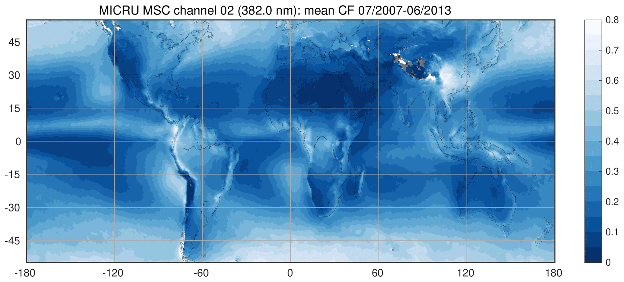
Figure F1The 6-year average of MICRU MSC channel 2 cloud fraction measurements recorded between 1 July 2007 and 30 June 2013. Areas without data are plotted in gray.
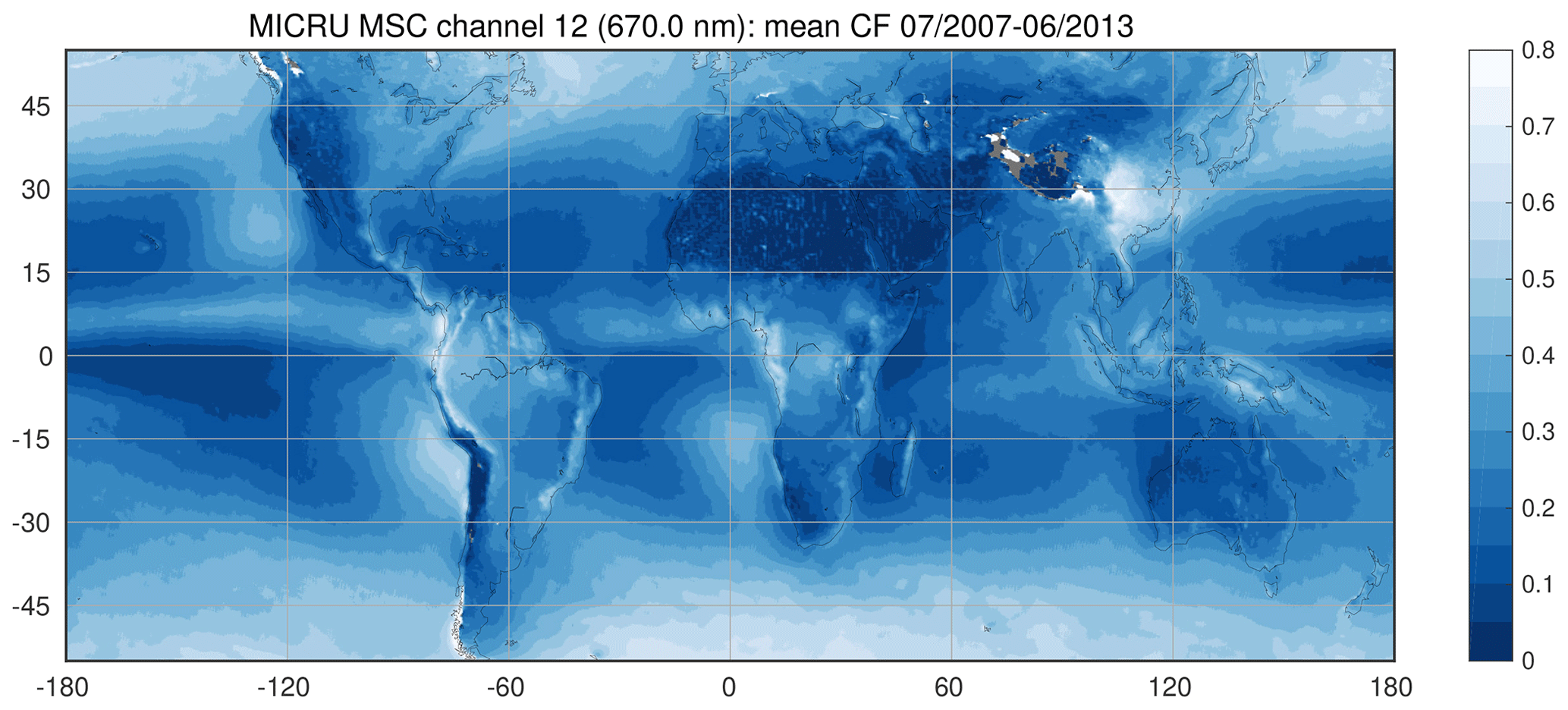
Figure F2The 6-year average of MICRU MSC channel 12 cloud fraction measurements recorded between 1 July 2007 and 30 June 2013. Areas without data are plotted in gray.
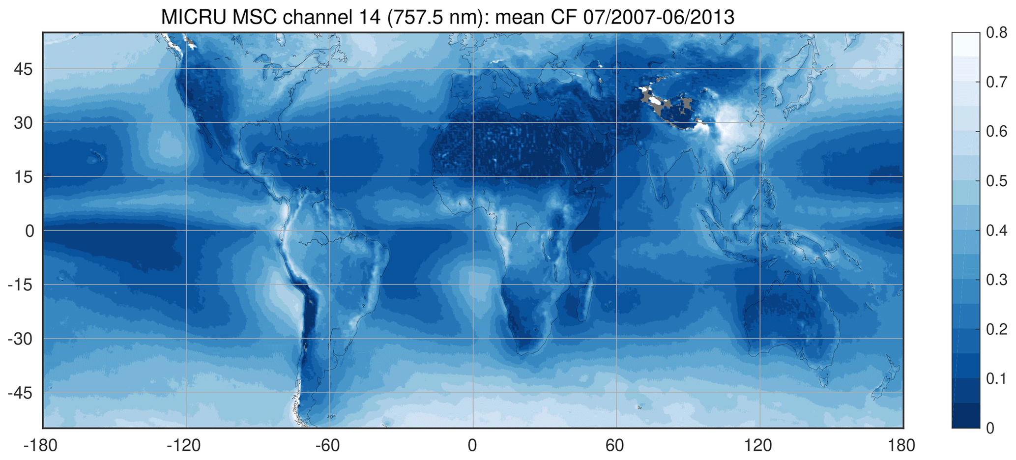
Figure F3The 6-year average of MICRU MSC channel 14 cloud fraction measurements recorded between 1 July 2007 and 30 June 2013. Areas without data are plotted in gray.
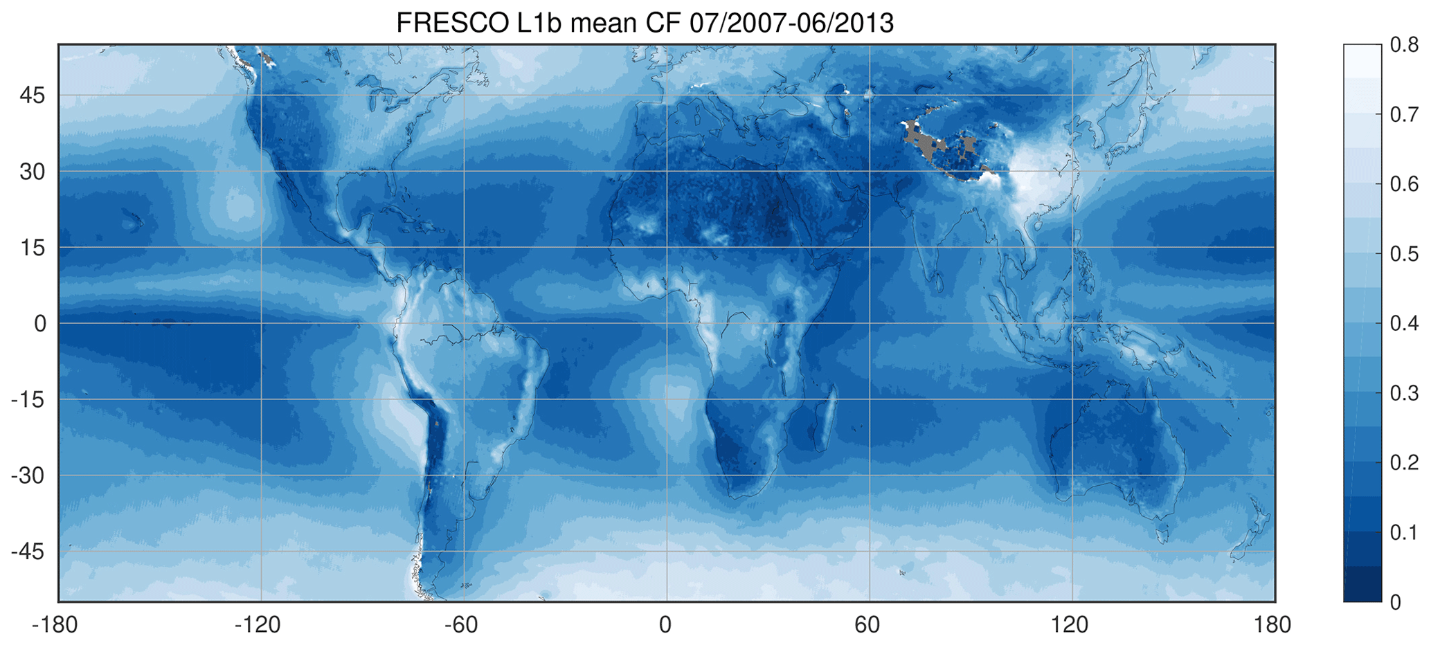
Figure F4Same as Fig. 14 but showing the 6-year average of the FRESCO L1b cloud fraction measurements recorded between 1 July 2007 and 30 June 2013. Areas without data are plotted in gray.
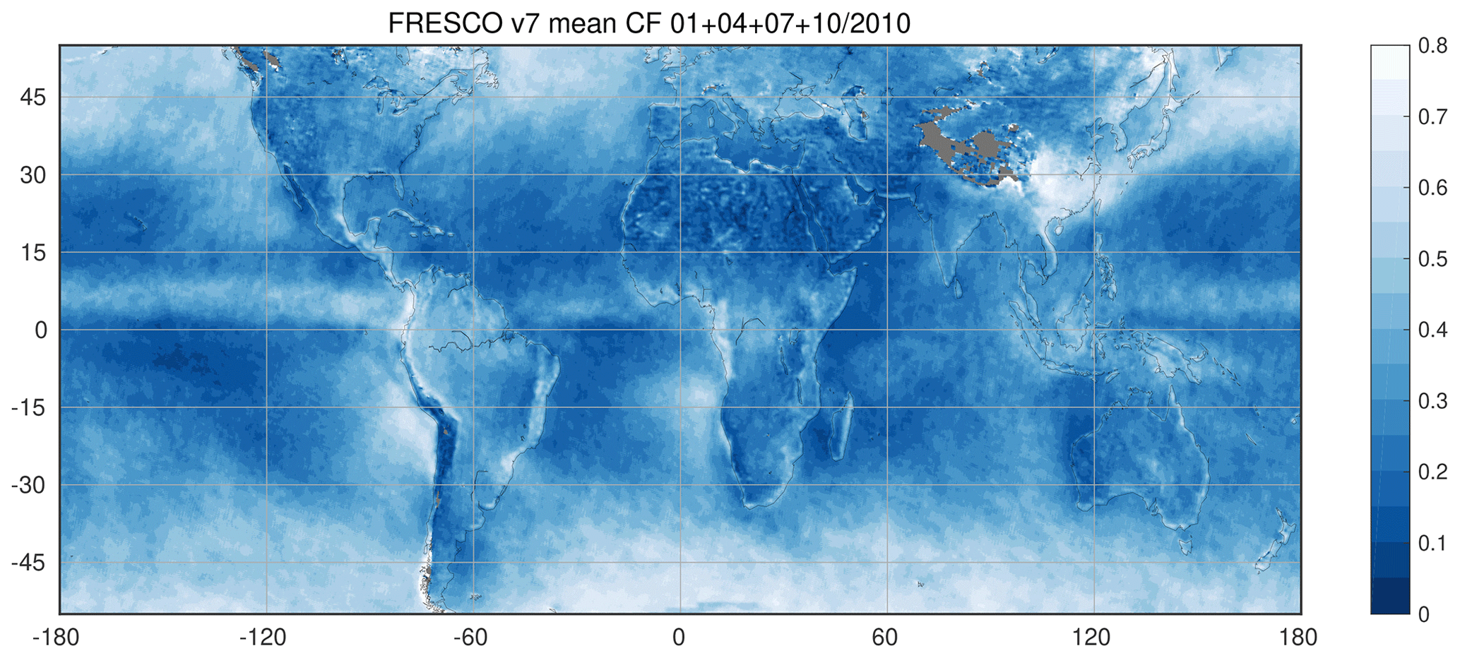
Figure F5Same as Fig. 14 but showing the 4-month average of the FRESCO v7 cloud fraction measurements recorded in January, April, July, and October 2010. Areas without data are plotted in gray.
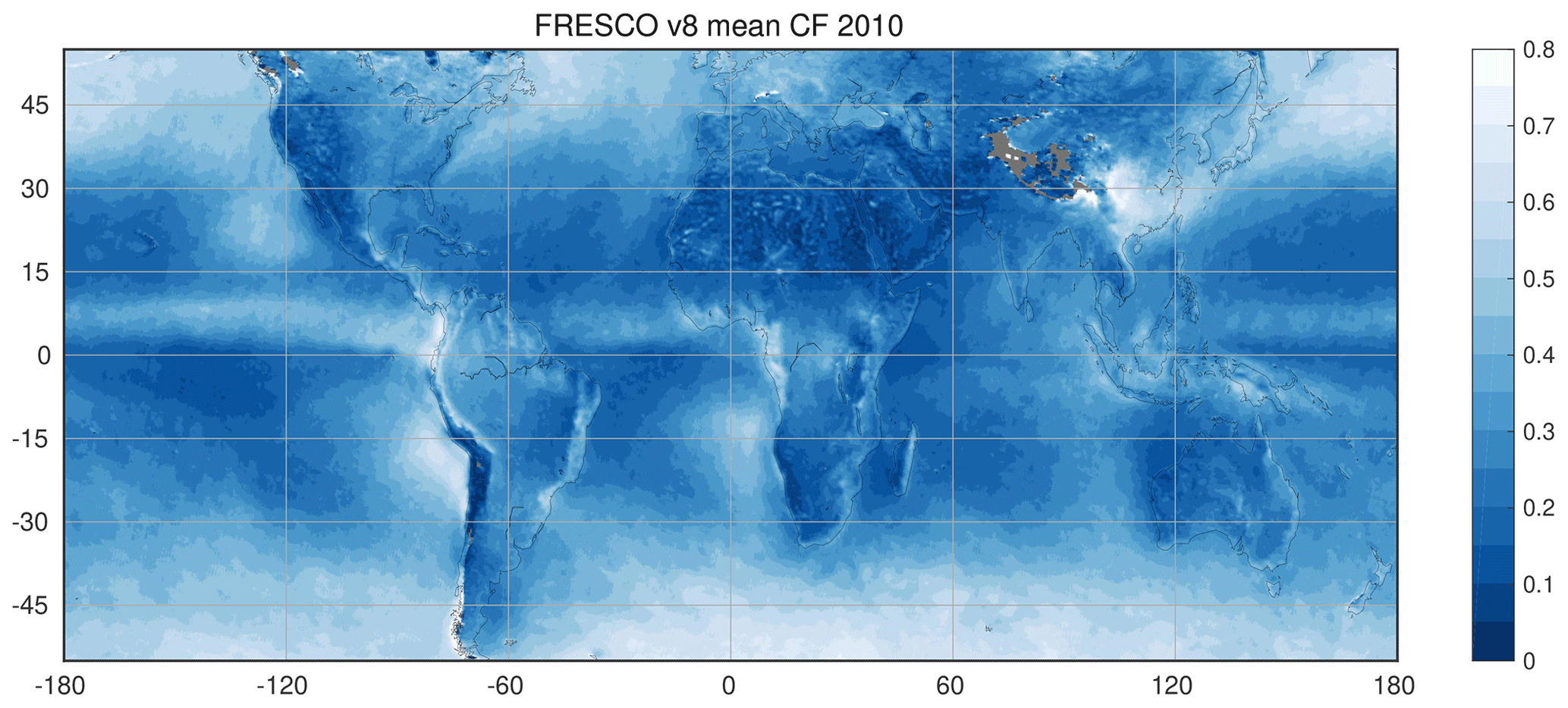
Figure F6Same as Fig. 14 but showing the 1-year average of the FRESCO v8 cloud fraction measurements recorded in 2010. Areas without data are plotted in gray.
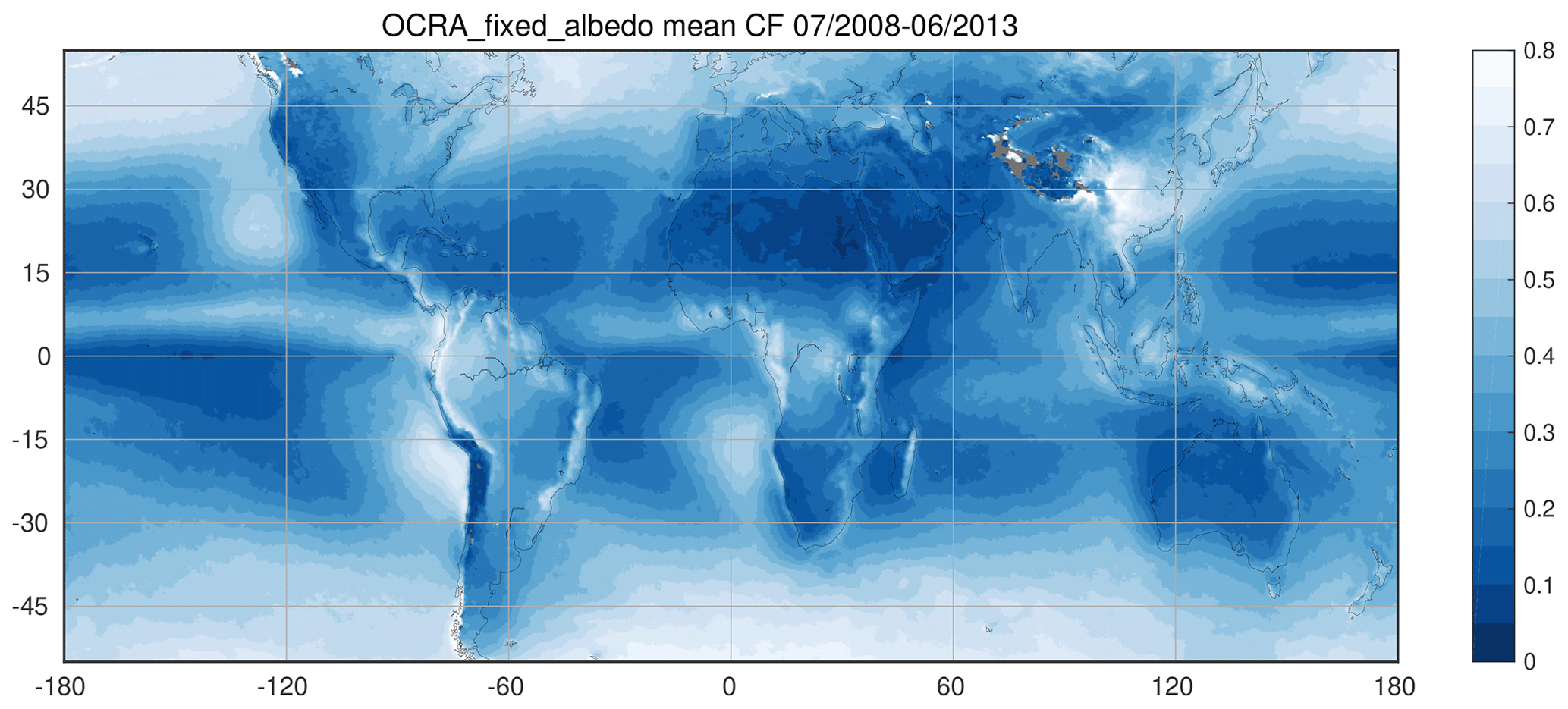
Figure F7Same as Fig. 14 but showing the 5-year average of the OCRA_fixed_albedo cloud fraction measurements recorded between 1 July 2008 and 30 June 2013. Areas without data are plotted in gray.
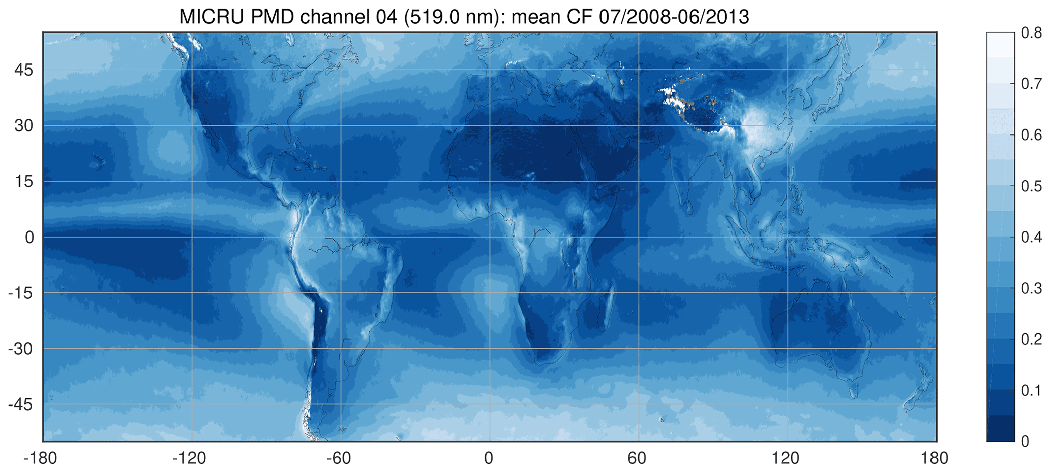
Figure F8Same as Fig. 14 but showing the 5-year average of the MICRU PMD channel 4 cloud fraction measurements recorded between 1 July 2008 and 30 June 2013. Areas without data are plotted in gray.

Figure F9Same as Fig. 14 but showing the 5-year average of the OCRA cloud fraction measurements recorded between 1 July 2008 and 30 June 2013. Areas without data are plotted in gray.
GOME-2 Level 1b data are available via the EUMETSAT Data Centre on the EUMETSAT Earth Observation (EO) Portal (see also https://navigator.eumetsat.int/product/EO:EUM:DAT:METOP:GOMEL1, last access: 25 May 2021). Reprocessed GOME-2 AAI data (R1) version 1.01 are available from AC-SAF (https://doi.org/10.15770/EUM_SAF_O3M_0003, AC SAF, 2017a; https://doi.org/10.15770/EUM_SAF_O3M_0004, AC SAF, 2017b). MODIS snow data have been provided by Hall and Riggs (2016) (https://doi.org/10.5067/MODIS/MOD10C2.006). Sea ice data have been provided by Cavalieri et al. (1996) (https://doi.org/10.5067/8GQ8LZQVL0VL). The Global 30-Arc-Second Elevation (GTOPO30) data set can be found at https://doi.org/10.5066/F7DF6PQS (USGS, 2018). The Global Self-consistent, Hierarchical, High-resolution Geography Database (GSHHG) can be downloaded from NOAA NCEI (https://www.ngdc.noaa.gov/mgg/shorelines/, NOAA, 2018). ERA-Interim data used in this study were provided by ECMWF. MICRU MSC results are archived and will be distributed through the Edmond service of the Max Planck Digital Library (https://edmond.mpdl.mpg.de/imeji/, last access: 27 May 2021) under https://doi.org/10.17617/3.59 (Sihler and Wagner, 2020). MICRU PMD results are available from the authors upon request.
HS developed and implemented the algorithm with additional input from MGPdV, SB, SD, CB, SW, and TW; SCIATRAN RT simulations were supervised by MGPdV; HS, MGPdV, CH, SB, and TW interpreted the results, HS drafted the paper; all co-authors were involved in proofing the paper.
The authors declare that they have no conflict of interest.
We thank Michael Grzegorski, the main developer of HICRU, for inspiration and discussion, and Andreas Richter (IUP Bremen) for fruitful discussions and the first application of the data. Furthermore, Piet Stammes (KNMI), Ping Wang (KNMI), Ronny Lutz (DLR), Diego Loyola (DLR), and Rüdiger Lang (EUMETSAT) are gratefully acknowledged. EUMETSAT and NASA are acknowledged for providing data. The programme developers at IUP/IFE Bremen are acknowledged for providing the SCIATRAN software.
This research has been supported by DLR Bonn (contract
no. 550EE1247) as part of the S5P/TROPOMI verification and by
ESA (contract no. ST-ESA-S5L2PP-CON-003) as part of
the Sentinel-5 verification.
The article processing charges for this open-access
publication were covered by the Max Planck Society.
This paper was edited by Andrew Sayer and reviewed by two anonymous referees.
AC SAF: GOME-2A Absorbing Aerosol Index MSC (R1) – Metop, EUMETSAT SAF on Atmospheric Composition Monitoring, https://doi.org/10.15770/EUM_SAF_O3M_0003, 2017a. a
AC SAF: GOME-2A Absorbing Aerosol Index PMD (R1) – Metop, EUMETSAT SAF on Atmospheric Composition Monitoring, https://doi.org/10.15770/EUM_SAF_O3M_0004, 2017b. a
Ahmad, Z., Bhartia, P. K., and Krotkov, N.: Spectral properties of backscattered UV radiation in cloudy atmospheres, J. Geophys. Res., 109, D01201, https://doi.org/10.1029/2003JD003395, 2004. a
Barkley, M. P., Kurosu, T. P., Chance, K., De Smedt, I., Van Roozendael, M., Arneth, A., Hagberg, D., and Guenther, A.: Assessing sources of uncertainty in formaldehyde air mass factors over tropical South America: Implications for top-down isoprene emission estimates, J. Geophys. Res., 117, 2156–2202, https://doi.org/10.1029/2011JD016827, 2012. a
Blum, M., Rozanov, V. V., Burrows, J. P., and Bracher, A.: Coupled ocean-atmosphere radiative transfer model in the framework of software package SCIATRAN: Selected comparisons to model and satellite data, Adv. Space Res., 49, 1728–1742, https://doi.org/10.1016/j.asr.2012.02.012, 2012. a
Boersma, K. F., Eskes, H. J., and Brinksma, E. J.: Error analysis for tropospheric NO2 retrieval from space, J. Geophys. Res., 109, D04311, https://doi.org/10.1029/2003JD003962, 2004. a
Bovensmann, H., Burrows, J. P., Buchwitz, M., Frerick, J., Noël, S., Rozanov, V. V., Chance, K. V., and Goede, A. P. H.: SCIAMACHY: mission objectives and measurement modes, J. Atmos. Sci., 56, 127–150, https://doi.org/10.1175/1520-0469(1999)056<0127:SMOAMM>2.0.CO;2, 1999. a
Burrows, J. P., Weber, M., Buchwitz, M., Rozanov, V., Ladstätter-Weißenmayer, A., Richter, A., DeBeek, R., Hoogen, R., Bramstedt, K., Eichmann, K.-U., Eisinger, M., and Perner, D.: The Global Ozone Monitoring Experiment (GOME): Mission concept and first scientific results, J. Atmos. Sci., 56, 151–175, https://doi.org/10.1175/1520-0469(1999)056<0151:TGOMEG>2.0.CO;2, 1999. a
Callies, J., Corpaccioli, E., Eisinger, M., Hahne, A., and Lefebvre, A.: GOME-2 – MetOp's Second-Generation Sensor for Operational Ozone Monitoring, ESA Bull.-Eur. Space, 102, 28–36, 2000. a
Cantrell, C. A.: Technical Note: Review of methods for linear least-squares fitting of data and application to atmospheric chemistry problems, Atmos. Chem. Phys., 8, 5477–5487, https://doi.org/10.5194/acp-8-5477-2008, 2008. a
Cavalieri, D. J., Parkinson, C. L., Gloersen, P., and Zwally, H. J.: Sea Ice Concentrations from Nimbus-7 SMMR and DMSP SSM/I-SSMIS Passive Microwave Data, Version 1, NSIDC-0051, 2007–2013, NASA National Snow and Ice Data Center Distributed Active Archive Center, Boulder, Colorado USA, https://doi.org/10.5067/8GQ8LZQVL0VL, 1996. a, b, c
Coleman, T. F. and Li, Y.: On the Convergence of Reflective Newton Methods for Large-Scale Nonlinear Minimization Subject to Bounds, Math. Program., 67, 189–224, https://doi.org/10.1007/BF01582221, 1994. a
Coleman, T. F. and Li, Y.: An Interior, Trust Region Approach for Nonlinear Minimization Subject to Bounds, SIAM J. Optimiz., 6, 418–445, https://doi.org/10.1137/0806023, 1996. a
Cox, C. and Munk, W.: Measurement Of The Roughness Of The Sea Surface From Photographs Of The Sun's Glitter, J. Opt. Soc. Am., 44, 838–850, 1954a. a, b, c, d
Cox, C. and Munk, W. H.: Statistics of the sea surface derived from sun glitter, J. Mar. Res., 13, 198–227, 1954b. a
Cracknell, A.: The Advanced Very High Resolution Radiometer, Taylor and Francis, London, UK, ISBN 9780748402090, 1997. a
Dee, D. P., Uppala, S. M., Simmons, A. J., Berrisford, P., Poli, P., Kobayashi, S., Andrae, U., Balmaseda, M. A., Balsamo, G., Bauer, P., Bechtold, P., Beljaars, A. C. M., van de Berg, L., Bidlot, J., Bormann, N., Delsol, C., Dragani, R., Fuentes, M., Geer, A. J., Haimberger, L., Healy, S. B., Hersbach, H., Hólm, E. V., Isaksen, L., Kållberg, P., Köhler, M., Matricardi, M., McNally, A. P., Monge-Sanz, B. M., Morcrette, J.-J., Park, B.-K., Peubey, C., de Rosnay, P., Tavolato, C., Thépaut, J.-N., and Vitart, F.: The ERA-Interim reanalysis: configuration and performance of the data assimilation system, Q. J. Roy. Meteor. Soc., 137, 553–597, https://doi.org/10.1002/qj.828, 2011. a, b
de Graaf, M., Sihler, H., Tilstra, L. G., and Stammes, P.: How big is an OMI pixel?, Atmos. Meas. Tech., 9, 3607–3618, https://doi.org/10.5194/amt-9-3607-2016, 2016. a, b
De Smedt, I., Müller, J.-F., Stavrakou, T., van der A, R., Eskes, H., and Van Roozendael, M.: Twelve years of global observations of formaldehyde in the troposphere using GOME and SCIAMACHY sensors, Atmos. Chem. Phys., 8, 4947–4963, https://doi.org/10.5194/acp-8-4947-2008, 2008. a
Desmons, M., Wang, P., Stammes, P., and Tilstra, L. G.: FRESCO-B: a fast cloud retrieval algorithm using oxygen B-band measurements from GOME-2, Atmos. Meas. Tech., 12, 2485–2498, https://doi.org/10.5194/amt-12-2485-2019, 2019. a
Deutschmann, T., Beirle, S., Frieß, U., Grzegorski, M., Kern, C., Kritten, L., Platt, U., Prados-Román, C., Pukite, J., Wagner, T., Werner, B., and Pfeilsticker, K.: The Monte Carlo atmospheric radiative transfer model McArtim: Introduction and validation of Jacobians and 3D features, J. Quant. Spectrosc. Ra., 112, 1119–1137, https://doi.org/10.1016/j.jqsrt.2010.12.009, 2011. a
Ebuchi, N. and Kizu, S.: Probability Distribution of Surface Wave Slope Derived Using Sun Glitter Images from Geostationary Meteorological Satellite and Surface Vector Winds from Scatterometers, J. Oceanogr., 58, 477–486, https://doi.org/10.1023/A:1021213331788, 2002. a, b
EUMETSAT: AVHRR Level 1b Product Guide, Doc.No.: EUM/OPS-EPS/MAN/04/0029, Issue: v3A, available at: https://www-cdn.eumetsat.int/files/2020-04/pdf_avhrr_l1b_product_guide.pdf (last access: 11 April 2021), 2011. a, b
EUMETSAT: GOME-2/Metop-A instrument, PPF and auxiliary-data change history, available at: http://oiswww.eumetsat.org/epsreports/html/history/MetopAGOME2PPFhist.pdf (last access: 22 May 2019), 2014. a
EUMETSAT: GOME-2 Factsheet, available at: http://www.eumetsat.int/ (last access: January 2019), 2015. a, b, c, d, e, f, g
Fasnacht, Z., Vasilkov, A., Haffner, D., Qin, W., Joiner, J., Krotkov, N., Sayer, A. M., and Spurr, R.: A geometry-dependent surface Lambertian-equivalent reflectivity product for UV–Vis retrievals – Part 2: Evaluation over open ocean, Atmos. Meas. Tech., 12, 6749–6769, https://doi.org/10.5194/amt-12-6749-2019, 2019. a
Fournier, N., Stammes, P., de Graaf, M., van der A, R., Piters, A., Grzegorski, M., and Kokhanovsky, A.: Improving cloud information over deserts from SCIAMACHY Oxygen A-band measurements, Atmos. Chem. Phys., 6, 163–172, https://doi.org/10.5194/acp-6-163-2006, 2006. a
Grainger, J. F. and Ring, J.: Anomalous Fraunhofer Line Profiles, Nature, 193, 762, https://doi.org/10.1038/193762a0, 1962. a
Grzegorski, M.: Cloud retrieval from UV/VIS satellite instruments (SCIAMACHY and GOME), Dissertation, University of Heidelberg, https://doi.org/10.11588/heidok.00010423, 2009. a
Grzegorski, M., Wenig, M., Platt, U., Stammes, P., Fournier, N., and Wagner, T.: The Heidelberg iterative cloud retrieval utilities (HICRU) and its application to GOME data, Atmos. Chem. Phys., 6, 4461–4476, https://doi.org/10.5194/acp-6-4461-2006, 2006. a, b, c, d, e, f, g
Hall, D. K. and Riggs, G. A.: MODIS/Terra Snow Cover 8-Day L3 Global 0.05Deg CMG, Version 6, 2007–2013, NASA National Snow and Ice Data Center Distributed Active Archive Center, Boulder, Colorado USA, https://doi.org/10.5067/MODIS/MOD10C2.006, 2016. a, b, c
Harmel, T. and Chami, M.: Estimation of the sunglint radiance field from optical satellite imagery over open ocean: multidirectional approach and polarization aspects, J. Geophys. Res.-Oceans, 118, 76–90, https://doi.org/10.1029/2012JC008221, 2013. a
Herman, J. R. and Celarier, E. A.: Earth surface reflectivity climatology at 340–380 nm from TOMS data, J. Geophys. Res., 102, 28003–28012, https://doi.org/10.1029/97JD02074, 1997. a
IFE-Bremen: User's Guide for the Software Package SCIATRAN (Radiative Transfer Model and Retrieval Algorithm) – Version 3.8, Internet, Institute of Remote Sensing (IFE), University of Bremen, Germany, available at: http://www.iup.uni-bremen.de/sciatran/free_downloads/users_guide_sciatran.pdf (last access: 14 February 2019), 2018. a
Justice, C., Vermote, E., Townshend, J., Defries, R., Roy, D., Hall, D., Salomonson, V., Privette, J., Riggs, G., Strahler, A., Lucht, W., Myneni, R., Knyazikhin, Y., Running, S., Nemani, R., Wan, Z., Huete, A., van Leeuwen, W., Wolfe, R., Giglio, L., Muller, J., Lewis, P., and Barnsley, M.: The Moderate Resolution Imaging Spectroradiometer (MODIS): land remote sensing for global change research, IEEE T. Geosci. Remote., 36, 1228–1249, https://doi.org/10.1109/36.701075, 1998. a
Kleipool, Q. L., Dobber, M. R., de Haan, J. F., and Levelt, P. F.: Earth surface reflectance climatology from 3 years of OMI data, J. Geophys. Res.-Atmos., 113, D18308, https://doi.org/10.1029/2008JD010290, 2008. a
KNMI: OMI Instrument Characteristics, available at: https://projects.knmi.nl/omi/research/instrument/characteristics.php (last access: 4 February 2015), 2019. a
Koelemeijer, R. B. A., Stammes, P., Hovenier, J. W., and de Haan, J. F.: A fast method for retrieval of cloud parameters using oxygen A-band measurements from Global Ozone Monitoring Experiment, J. Geophys. Res., 106, 3475–3490, https://doi.org/10.1029/2000JD900657, 2001. a, b, c
Koelemeijer, R. B. A., de Haan, J. F., and Stammes, P.: A database of spectral surface reflectivity in the range 335–772 nm derived from 5.5 years of GOME observations, J. Geophys. Res., 108, 4070, https://doi.org/10.1029/2002JD002429, 2003. a, b
Kokhanovsky, A. A., von Hoyningen-Huene, W., and Burrows, J. P.: Determination of the cloud fraction in the SCIAMACHY ground scene using MERIS spectral measurements,, Int. J. Remote Sens., 30, 6151–6167, https://doi.org/10.1080/01431160902842326, 2009. a
Krijger, J. M., van Weele, M., Aben, I., and Frey, R.: Technical Note: The effect of sensor resolution on the number of cloud-free observations from space, Atmos. Chem. Phys., 7, 2881–2891, https://doi.org/10.5194/acp-7-2881-2007, 2007. a, b
Kuze, A. and Chance, K. V.: Analysis of cloud top height and cloud coverage from satellites using the O2 A and B bands, J. Geophys. Res., 99, 14481–14491, https://doi.org/10.1029/94JD01152, 1994. a
Lang, R.: GOME-2 PMD Band Definitions 3.0 and PMD Calibration, EUMETSAT, Doc.No. EUM/OPS-EPS/DOC/07/0601, Issue v8, available at: https://www-cdn.eumetsat.int/files/2020-04/pdf_gome2_pmd_band_def_and_calib.pdf (last access: 11 April 2021), 2010. a, b
Levelt, P. F., van den Oord, G. H. J., Dobber, M. R., Malkki, A., Visser, H., de Vries, J., Stammes, P., Lundell, J. O. V., and Saari, H.: The Ozone Monitoring Instrument, IEEE T. Geosci. Remote, 44, 1093–1101, https://doi.org/10.1109/TGRS.2006.872333, 2006. a
Li, X. and Strahler, A. H.: Geometric-optical bidirectional reflectance modeling of the discrete crown vegetation canopy: effect of crown shape and mutual shadowing, IEEE T. Geosci. Remote, 30, 276–292, https://doi.org/10.1109/36.134078, 1992. a
Liu, C., Beirle, S., Butler, T., Liu, J., Hoor, P., Jöckel, P., Penning de Vries, M., Pozzer, A., Frankenberg, C., Lawrence, M. G., Lelieveld, J., Platt, U., and Wagner, T.: Application of SCIAMACHY and MOPITT CO total column measurements to evaluate model results over biomass burning regions and Eastern China, Atmos. Chem. Phys., 11, 6083–6114, https://doi.org/10.5194/acp-11-6083-2011, 2011. a
Lorente, A., Folkert Boersma, K., Yu, H., Dörner, S., Hilboll, A., Richter, A., Liu, M., Lamsal, L. N., Barkley, M., De Smedt, I., Van Roozendael, M., Wang, Y., Wagner, T., Beirle, S., Lin, J.-T., Krotkov, N., Stammes, P., Wang, P., Eskes, H. J., and Krol, M.: Structural uncertainty in air mass factor calculation for NO2 and HCHO satellite retrievals, Atmos. Meas. Tech., 10, 759–782, https://doi.org/10.5194/amt-10-759-2017, 2017. a, b
Lorente, A., Boersma, K. F., Stammes, P., Tilstra, L. G., Richter, A., Yu, H., Kharbouche, S., and Muller, J.-P.: The importance of surface reflectance anisotropy for cloud and NO2 retrievals from GOME-2 and OMI, Atmos. Meas. Tech., 11, 4509–4529, https://doi.org/10.5194/amt-11-4509-2018, 2018. a, b, c, d, e, f
Loyola, D.: A new cloud recognition algorithm for optical sensors, in: IGARSS '98. Sensing and Managing the Environment. 1998 IEEE International Geoscience and Remote Sensing. Symposium Proceedings (Cat. No.98CH36174), 6–10 July 1998, Seattle, USA, 97-80873, IEEE, 572–574, https://doi.org/10.1109/IGARSS.1998.699514, 1998. a
Loyola, D., Thomas, W., Livschitz, Y., Ruppert, T., Albert, P., and Hollmann, R.: Cloud Properties Derived From GOME/ERS-2 Backscatter Data for Trace Gas Retrieval, IEEE T. Geosci. Remote, 45, 2747–2758, https://doi.org/10.1109/TGRS.2007.901043, 2007. a, b
Loyola, D., Koukouli, M., Valks, P., Balis, D., Hao, N., Van Roozendael, M., Spurr, R., Zimmer, W., Kiemle, S., Lerot, C., and Lambert, J.-C.: The GOME-2 Total Column Ozone Product: Retrieval Algorithm and Ground-Based Validation, J. Geophys. Res, 116, D07302, https://doi.org/10.1029/2010JD014675, 2011. a
Loyola, D. G., Gimeno García, S., Lutz, R., Argyrouli, A., Romahn, F., Spurr, R. J. D., Pedergnana, M., Doicu, A., Molina García, V., and Schüssler, O.: The operational cloud retrieval algorithms from TROPOMI on board Sentinel-5 Precursor, Atmos. Meas. Tech., 11, 409–427, https://doi.org/10.5194/amt-11-409-2018, 2018. a, b, c, d
Loyola, D. G., Xu, J., Heue, K.-P., and Zimmer, W.: Applying FP_ILM to the retrieval of geometry-dependent effective Lambertian equivalent reflectivity (GE_LER) daily maps from UVN satellite measurements, Atmos. Meas. Tech., 13, 985–999, https://doi.org/10.5194/amt-13-985-2020, 2020. a
Lutz, R., Loyola, D., Gimeno García, S., and Romahn, F.: OCRA radiometric cloud fractions for GOME-2 on MetOp-A/B, Atmos. Meas. Tech., 9, 2357–2379, https://doi.org/10.5194/amt-9-2357-2016, 2016. a, b, c, d, e, f, g
Martin, J., Eugenio, F., Marcello, J., and Medina, A.: Automatic Sun Glint Removal of Multispectral High-Resolution Worldview-2 Imagery for Retrieving Coastal Shallow Water Parameters, Remote Sens., 8, 37, https://doi.org/10.3390/rs8010037, 2016. a
Martin, R. V., Chance, K., Jacob, D., Kurosu, T. P., Spurr, R. J. D., Bucsela, E., Gleason, J. F., Palmer, P. I., Bey, I., Fiore, A. M., Li, Q., Yantosca, R. M., and Koelemeijer, R. B. A.: An improved retrieval of tropospheric nitrogen dioxide from GOME, J. Geophys. Res., 107, 4437, https://doi.org/10.1029/2001JD001027, 2002. a
McKenzie, R. L., Johnston, P. V., McElroy, C. T., Kerr, J. B., and Solomon, S.: Altitude distributions of stratospheric constituents from ground‐based measurements at twilight, J. Geophys. Res.-Atmos., 96, 15499–15511, https://doi.org/10.1029/91JD01361, 1991. a
McPeters, R., Bhartia, P. K., Krueger, A. J., Herman, J. R., Schlesinger, B. M., Wellemeyer, C. G., Seftor, C. J., Jaross, G., Taylor, S. L., Swissler, T., Torres, O., Labow, G., Byerly, W., and Cebula, R. P.: Nimbus-7 Total Ozone Mapping Spectrometer (TOMS) Data Products User’s Guide, Nasa reference publication 138, NASA, available at: https://ozoneaq.gsfc.nasa.gov/media/docs/epusrguide.pdf (last access: 17 November 2020), 1996. a, b
Munro, R., Eisinger, M., Anderson, C., Callies, J., Corpaccioli, E., Lang, R., Lefebvre, A., Livschitz, Y., and Albiñana, A. P.: GOME-2 on MetOp, in: Proc. of The 2006 EUMETSAT Meteorological Satellite Conference, 12–16 June 2006, Helsinki, Finland, EUMETSAT, p. 48, 2006. a
Munro, R., Lang, R., Klaes, D., Poli, G., Retscher, C., Lindstrot, R., Huckle, R., Lacan, A., Grzegorski, M., Holdak, A., Kokhanovsky, A., Livschitz, J., and Eisinger, M.: The GOME-2 instrument on the Metop series of satellites: instrument design, calibration, and level 1 data processing – an overview, Atmos. Meas. Tech., 9, 1279–1301, https://doi.org/10.5194/amt-9-1279-2016, 2016. a, b, c, d, e, f
NOAA: Global Self-consistent Hierarchical High-resolution Geography (GSHHG), Version 2.3.7 June 15, 2017, available at: https://www.ngdc.noaa.gov/mgg/shorelines/, last access: 1 March 2018. a, b, c
NOAA: Advanced Very High Resolution Radiometer – AVHRR, available at: https://www.avl.class.noaa.gov/release/data_available/avhrr/index.htm, last access: 11 April 2021. a
Noguchi, K., Richter, A., Rozanov, V., Rozanov, A., Burrows, J. P., Irie, H., and Kita, K.: Effect of surface BRDF of various land cover types on geostationary observations of tropospheric NO2, Atmos. Meas. Tech., 7, 3497–3508, https://doi.org/10.5194/amt-7-3497-2014, 2014. a
Noxon, J. F., Whipple, E. C., and Hyde, R. S.: Stratospheric NO2 – 1. Observational method and behaviour at mid-latitude, J. Geophys. Res., 84, 5047–5076, https://doi.org/10.1029/JC084iC08p05047, 1979. a
Perliski, L. and Solomon, S.: On the evaluation of air mass factors for atmospheric near-ultraviolet and visible absorption spectroscopy, J. Geophys. Res., 98, 10363–10374, https://doi.org/10.1029/93JD00465, 1993. a
Popp, C., Wang, P., Brunner, D., Stammes, P., Zhou, Y., and Grzegorski, M.: MERIS albedo climatology for FRESCO+ O2 A-band cloud retrieval, Atmos. Meas. Tech., 4, 463–483, https://doi.org/10.5194/amt-4-463-2011, 2011. a, b
Rozanov, V. V. and Rozanov, A. V.: Differential optical absorption spectroscopy (DOAS) and air mass factor concept for a multiply scattering vertically inhomogeneous medium: theoretical consideration, Atmos. Meas. Tech., 3, 751–780, https://doi.org/10.5194/amt-3-751-2010, 2010. a
Rozanov, V. V., Rozanov, A. V., Kokhanovsky, A. A., and Burrows, J. P.: Radiative transferthrough terrestrial atmosphere and ocean: Software package SCIATRAN, J. Quant. Spectrosc. Ra., 113, 13–71, https://doi.org/10.1016/j.jqsrt.2013.07.004, 2014. a
Sarkissian, A., Roscoe, H. K., and Fish, D. J.: Ozone measurementsby zenith-sky spectrometers: an evaluation of errors in air-massfactors calculated by radiative transfer model, J. Quant. Spectrosc. Ra., 54, 471–480, https://doi.org/10.1016/0022-4073(95)00085-Y, 1995. a
Schueler, C. F., Clement, J. E., Ardanuy, P. E., Welsch, C., DeLuccia, F., and Swenson, H.: NPOESS VIIRS sensor design overview, Proc. SPIE 4483, in: Earth Observing Systems VI, https://doi.org/10.1117/12.453451, 2002. a
Sihler, H. and Wagner, T.: MICRU effective cloud fractions from GOME-2A, Max Planck Digital Library, https://doi.org/10.17617/3.59, 2020. a
Sihler, H., Lübcke, P., Lang, R., Beirle, S., de Graaf, M., Hörmann, C., Lampel, J., Penning de Vries, M., Remmers, J., Trollope, E., Wang, Y., and Wagner, T.: In-operation field-of-view retrieval (IFR) for satellite and ground-based DOAS-type instruments applying coincident high-resolution imager data, Atmos. Meas. Tech., 10, 881–903, https://doi.org/10.5194/amt-10-881-2017, 2017. a, b, c, d
Solomon, S., Schmeltekopf, A. L., and Sanders, R. W.: On the interpretation of zenith sky absorption measurements, J. Geophys. Res.-Atmos., 92, 8311–8319, https://doi.org/10.1029/JD092iD07p08311, 1987. a, b
Stammes, P., Sneep, M., de Haan, J. F., Veefkind, J. P., Wang, P., and Levelt, P. F.: Effective cloud fractions from the Ozone Monitoring Instrument: Theoretical framework and validation, J. Geophys. Res.-Atmos., 113, D16S38, https://doi.org/10.1029/2007JD008820, 2008. a, b, c
TEMIS: FRESCO product versions description, available at: https://www.temis.nl/fresco/versions.php, last access: 15 May 2021. a, b, c
Tilstra, L. G., De Graaf, M., Aben, I., and Stammes, P.: In‐flight degradation correction of SCIAMACHY UV reflectances and Absorbing Aerosol Index, J. Geophys. Res.-Atmos., 117, D06209, https://doi.org/10.1029/2011JD016957, 2012. a
Tilstra, L. G., Tuinder, O. N. E., and Stammes, P.: Algorithm theoretical basis document – GOME-2 surface LER product, available at: https://acsaf.org/docs/atbd/Algorithm_Theoretical_Basis_Document_LER_Mar_2019.pdf (last access: 15 May 2021), 2017a. a
Tilstra, L. G., Tuinder, O. N. E., Wang, P., and Stammes, P.: Surface reflectivity climatologies from UV to NIR determined from Earth observations by GOME-2 and SCIAMACHY, J. Geophys. Res.-Atmos., 122, 4084–4111, https://doi.org/10.1002/2016JD025940, 2017b. a, b, c, d
Tuinder, O. N. E., de Winter-Sorkina, R., and Builtjes, P. J. H.: Retrieval methods of effective cloud cover from the GOME instrument: an intercomparison, Atmos. Chem. Phys., 4, 255–273, https://doi.org/10.5194/acp-4-255-2004, 2004. a
Tuinder, O., de Graaf, M., Tilstra, G., Penning de Vries, M., and Kooreman, M.: Algorithm theoretical basis document – ATBD for the Absorbing Aerosol Index product, available at: https://acsaf.org/docs/atbd/Algorithm_Theoretical_Basis_Document_NAR_NAP_ARS_ARP_Sep_2019.pdf, last access: 28 November 2020. a, b
USGS: Global 30 Arc-Second Elevation (GTOPO30), Internet, USGS EROS Archive, https://doi.org/10.5066/F7DF6PQS, 2018. a, b, c
Várnai, T. and Marshak, A.: View angle dependence of cloud optical thicknesses retrieved by Moderate Resolution Imaging Spectroradiometer (MODIS), J. Geophys. Res., 112, D06203, https://doi.org/10.1029/2005JD006912, 2007. a
Vasilkov, A., Qin, W., Krotkov, N., Lamsal, L., Spurr, R., Haffner, D., Joiner, J., Yang, E.-S., and Marchenko, S.: Accounting for the effects of surface BRDF on satellite cloud and trace-gas retrievals: a new approach based on geometry-dependent Lambertian equivalent reflectivity applied to OMI algorithms, Atmos. Meas. Tech., 10, 333–349, https://doi.org/10.5194/amt-10-333-2017, 2017. a, b, c, d, e
Vasilkov, A., Yang, E.-S., Marchenko, S., Qin, W., Lamsal, L., Joiner, J., Krotkov, N., Haffner, D., Bhartia, P. K., and Spurr, R.: A cloud algorithm based on the O2-O2 477 nm absorption band featuring an advanced spectral fitting method and the use of surface geometry-dependent Lambertian-equivalent reflectivity, Atmos. Meas. Tech., 11, 4093–4107, https://doi.org/10.5194/amt-11-4093-2018, 2018. a, b
Veefkind, J. P., Aben, I., McMullan, K., Förster, H., de Vries, J., Otter, G., Claas, J., Eskes, H. J., de Haan, J. F., Kleipool, Q., van Weele, M., Hasekamp, O., Hoogeveen, R., Landgraf, J., Snel, R., Tol, P., Ingmann, P., Voors, R., Kruizinga, B., Vink, R., Visser, H., and Levelt, P. F.: TROPOMI on the ESA Sentinel-5 Precursor: A GMES mission for global observations of the atmospheric composition for climate, air quality and ozone layer applications, Remote Sens. Environ., 120, 70–83, https://doi.org/10.1016/j.rse.2011.09.027, 2012. a, b
Veefkind, J. P., de Haan, J. F., Sneep, M., and Levelt, P. F.: Improvements to the OMI O2–O2 operational cloud algorithm and comparisons with ground-based radar–lidar observations, Atmos. Meas. Tech., 9, 6035–6049, https://doi.org/10.5194/amt-9-6035-2016, 2016. a, b
Wagner, T., Heland, J., Zöger, M., and Platt, U.: A fast H2O total column density product from GOME – Validation with in-situ aircraft measurements, Atmos. Chem. Phys., 3, 651–663, https://doi.org/10.5194/acp-3-651-2003, 2003. a
Wang, P., Stammes, P., van der A, R., Pinardi, G., and van Roozendael, M.: FRESCO+: an improved O2 A-band cloud retrieval algorithm for tropospheric trace gas retrievals, Atmos. Chem. Phys., 8, 6565–6576, https://doi.org/10.5194/acp-8-6565-2008, 2008. a, b, c, d, e
Wang, P., Tuinder, O., and Stammes, P.: FRESCO+ version 2 for GOME-2 Metop-C processing, available at: http://www.temis.nl/fresco/frescopv2_metopc_WP1_report_20181026.pdf (last access: 25 May 2021), 2018. a
Wanner, W., Li, X., and Strahler, A. H.: On the derivation of kernels for kernel-driven models of bidirectional reflectance, J. Geophys. Res., 100, 21077–21089, https://doi.org/10.1029/95JD02371, 1995. a, b
Wessel, P. and Smith, W. H. F.: A Global Self-consistent, Hierarchical, High-resolution Shoreline Database, J. Geophys. Res., 101, 8741–8743, 1996. a, b
Zhang, H. and Wang, M.: Evaluation of sun glint models using MODIS measurements, J. Quant. Spectrosc. Ra., 111, 492–506, https://doi.org/10.1016/j.jqsrt.2009.10.001, 2010. a, b
- Abstract
- Introduction
- Method
- Results
- Discussion
- Conclusions
- Appendix A: Iterative surface fitting
- Appendix B: Tmin merging steps
- Appendix C: Tmin parameter map
- Appendix D: Wavelength dependency of MICRU results
- Appendix E: Matrix comparison between MICRU, FRESCO, and OCRA
- Appendix F: Global average cloud fractions
- Data availability
- Author contributions
- Competing interests
- Acknowledgements
- Financial support
- Review statement
- References