The SPARC Water Vapor Assessment II: assessment of satellite measurements of upper tropospheric humidity

Nineteen limb-viewing data sets (occultation, passive thermal, and UV scattering) and two nadir upper tropospheric humidity (UTH) data sets are intercompared and also compared to frost-point hygrometer balloon sondes. The upper troposphere considered here covers the pressure range from 300–100 hPa. UTH is a challenging measurement, because concentrations vary between 2–1000 ppmv (parts per million by volume), with sharp changes in vertical gradients near the tropopause. Cloudiness in this region also makes the measurement challenging. The atmospheric temperature is also highly variable ranging from 180–250 K. The assessment of satellite-measured UTH is based on coincident comparisons with balloon frost-point hygrometer sondes, multi-month mapped comparisons, zonal mean time series comparisons, and coincident satellite-to-satellite comparisons. While the satellite fields show similar features in maps and time series, quantitatively they can differ by a factor of 2 in concentration, with strong dependencies on the amount of UTH. Additionally, time-lag response-corrected Vaisala RS92 radiosondes are compared to satellites and the frost-point hygrometer measurements. In summary, most satellite data sets reviewed here show on average ∼30 % agreement amongst themselves and frost-point data but with an additional ∼30 % variability about the mean bias. The Vaisala RS92 sonde, even with a time-lag correction, shows poor behavior for pressures less than 200 hPa.

1 Introduction

A general assessment of water vapor measurements, both from remote and in situ sensors, was undertaken within the Stratosphere-troposphere Processes And their Role in Climate (SPARC) core project of the World Climate Research Programme (WCRP) prior to 2000. This activity known as the Water Vapor Assessment (WAVAS) published a report in 2000 (Kley et al., 2000). Since then, there has been a significant increase in the number of satellite missions, ground-based instruments, launches of balloon frost-point hygrometers (BFHs), and improved operational radiosonde hygrometers. Therefore, an assessment of these new resources is needed, now referred to as the SPARC WAVAS-II assessment. This paper amongst several in this ACP/AMT/ESSD special issue focuses on the upper troposphere. The upper troposphere is defined, depending on the application, from 300 hPa to the NASA Goddard's Global Modeling Assimilation Office (GMAO) Modern-Era Retrospective analysis for Research and Applications (MERRA) (Gelaro et al., 2017) tropopause height or 100 hPa.

2 Data sets

Table 1 lists the 25 satellite data sets (representing 16 instruments) that are considered in this report. In addition, we use BFH and corrected Vaisala RS92 radiosondes. Although BFHs have been in use for decades and launched from multiple sites, only six sites are considered here as they have a long time series of repeated launches. This helps provide some comparison statistics and temporal variability. The chosen sites are Boulder, USA (40.0^∘ N, 105.3^∘ W; 1980 to present); Lauder, New Zealand (45.0^∘ S, 169.7^∘ E; 2004 to present); Hilo, USA (19.7^∘ N, 155.1^∘ W; 2010 to present); Heredia, Costa Rica (10.0^∘ N, 84.1^∘ W; 2005 to present); Lindenberg, Germany (52.2^∘ N, 14.2^∘ E; 2006 to present); and Sodankylä, Finland (67.4^∘ N, 26.6^∘ E; 2002 to present). The Global Climate Observing System (GCOS) Reference Upper Air Network (GRUAN) launches high-quality radiosondes for climate research. Here we use water vapor observations from the Vaisala RS92 radiosondes, which have been processed by GRUAN to remove all known biases and to correct for all known effects influencing water vapor measurements (Dirksen et al., 2014). For the corrected Vaisala RS92 radiosonde set, we use data from Barrow Atmospheric Baseline Observatory (denoted Barrow hereafter), USA (71.3^∘ N, 156.3^∘ W; 2009 to present); Boulder, USA (40.0^∘ N, 105.3^∘ W; 2011 to present); Cabauw, the Netherlands (52.1^∘ N, 5.5^∘ E; 2011 to present); Lauder, New Zealand (45.0^∘ S, 169.7^∘ E; 2012 to present); Lindenberg, Germany (52.2^∘ N, 14.2^∘ E; 2005 to present); Ny-Ålesund, Norway (78.9^∘ N, 12.6^∘ E; 2006 to present); Southern Great Plains, USA (36.6^∘ N, 97.0^∘ W; 2009 to present); and Sodankylä, Finland (67.4^∘ N, 26.6^∘ E; 2007 to present). The locations of the balloon sites used in this study are shown in Fig. 1.

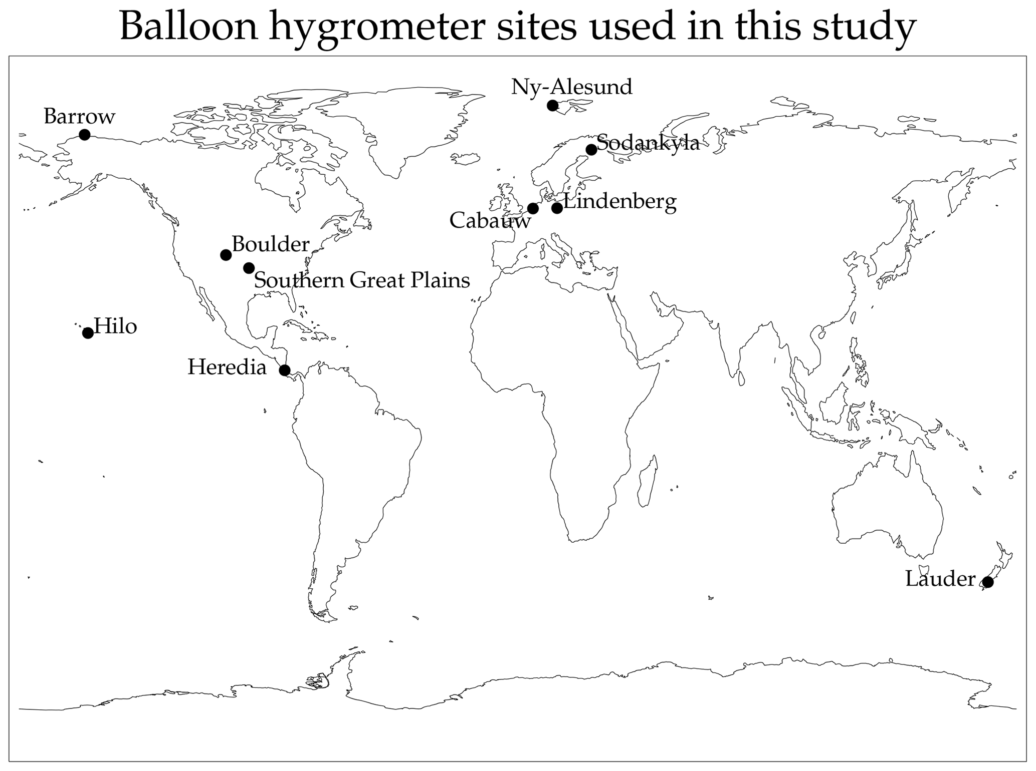
Figure 1 Balloon frost-point launch sites used in this study.

Aumann et al. (2003)Bernath (2017)Bertaux et al. (2000)Russell III et al. (1993)Gille et al. (2003)McElroy et al. (2007)Carlotti et al. (2001)Carlotti et al. (2001)Raspollini et al. (2006)Raspollini et al. (2006)Clarmann et al. (2003)Clarmann et al. (2009)Ridolfi et al. (2000)Ridolfi et al. (2000)Livesey et al. (2006)Read et al. (2001)Lumpe et al. (2002)Damadeo et al. (2013)Davis et al. (2020)Bovensmann et al. (1999)Kikuchi et al. (2010)Millan et al. (2013)Eriksson et al. (2014)Eriksson et al. (2014)Shephard et al. (2007)

Table 1 Data sets considered for upper tropospheric H₂O quality assessment.

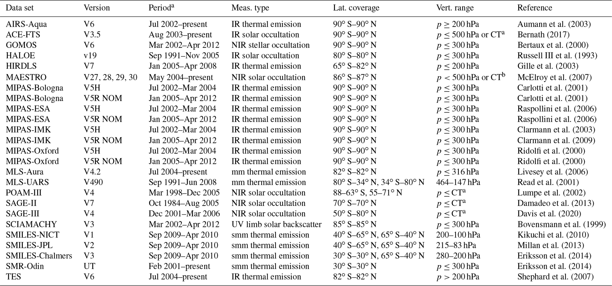
^a Comparisons are performed prior to 2017. ^b Cloud top (CT).

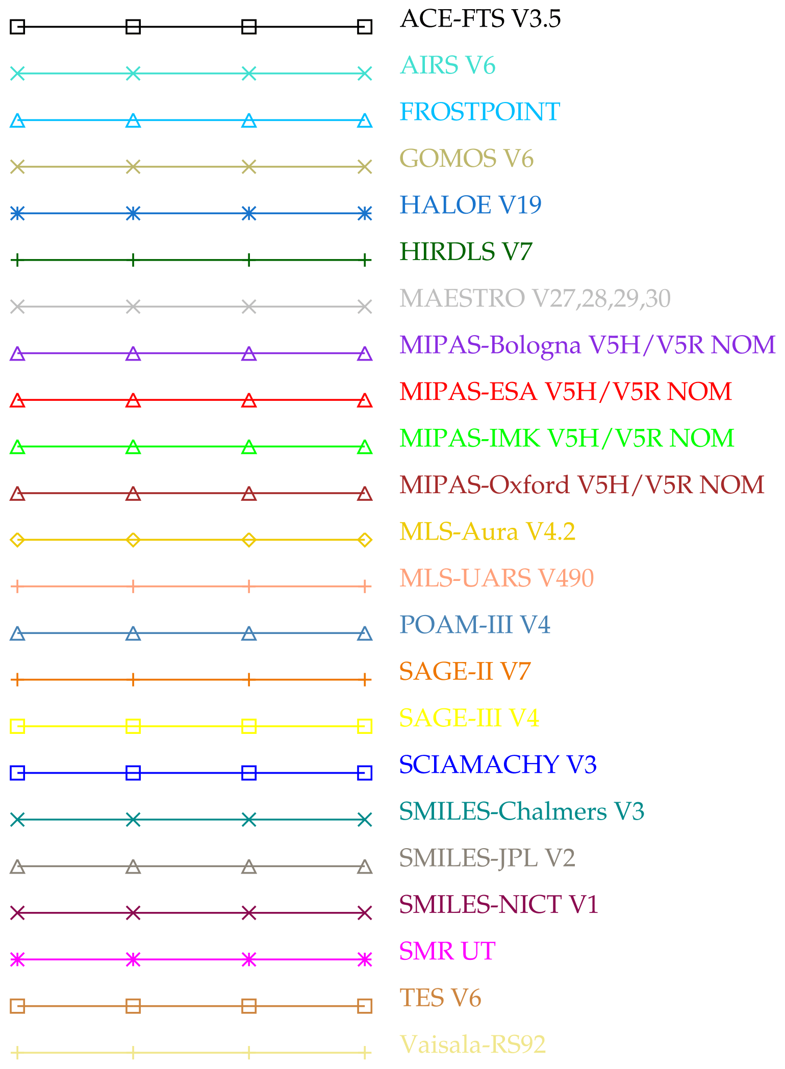
The satellite data sets are described in more detail in an overview paper by Walker and Stiller (2022). The data sets are quality screened as per recommendations from each of the data set providers. These data sets were read and repackaged in a common format that contains the following fields: year, UT time, longitude, latitude, day–night or sunrise–sunset flag, tropopause height, height, pressure, H₂O concentration, and H₂O concentration uncertainty in parts per million by volume (ppmv). Figure 2 shows a list of data sets used here, and the color and symbol coding is used when multiple data sets are shown in a plot.

Figure 2 The colors and symbols used to identify instruments in multi-instrument plots.

3 Comparison methods

Upper tropospheric humidity (UTH) is highly variable both temporally and spatially, making accuracy assessments difficult. Three comparison methods (coincident comparisons, time series, and gridded maps) are used here to assess the data. For coincident comparisons, we compare measurement pairs that are within 2.5^∘ in longitude and latitude and 3 h in time. The spatial coincidence is roughly the along-track weighting function width for a limb sounder (∼250 km), and there is no benefit to using a tighter criterion. The temporal matching criterion is rather arbitrary but is well under a diurnal time difference (12 h). For comparisons using a solar occultation satellite, the time and position coincidence is expanded to 8^∘ longitude, 2.5^∘ latitude, and 18 h. In principle, coincident pair matches are the best method of comparing two data sets but have some limitations: having a suitable number of coincidences to obtain enough statistics and, secondly, having good global coverage of the matches. For example, comparing two limb viewers in different sun-synchronous orbits means the only available coincidences will occur for specific latitudes where the local viewing time is within ±3 h of sunrise and sunset. The situation is even worse for comparing a sun-synchronous limb sounder to an occultation instrument, which is why the time window is considerably expanded for those comparisons.

Time series comparisons are useful to see how well the instruments track temporal changes and interannual variability. These comparisons are also useful for detecting possible drifts in their UTH retrievals (Livesey et al., 2021; Cebula et al., 1988). This is why we only used BFH sites that have frequent launches (monthly or more frequent) over several years.

The third comparison methodology compares gridded data maps. Many scientific studies are interested in global distributions of UTH during the year and also how this changes interannually (Chung et al., 2016; Schoeberl et al., 2013; Hegglin et al., 2013; Soden and Lanzante, 1996). One advantage of this type of comparison is that small-scale variability over time and space is averaged out. A disadvantage is that there can be significant sampling biases. For example, limb-viewing infrared (IR) instruments are heavily cloud contaminated in the tropics and will show a significant dry bias compared to maps made from nadir-viewing or submillimeter instruments (Millán et al., 2018). This study will show that the sampling bias is more than a factor of 2 in the upper troposphere. Also there will be temporal biases, because sun-synchronous orbiters only sample two local times, missing much of the diurnal cycle (Eriksson et al., 2010).

4 Comparing a coincident in situ measurement to a volume-averaged measurement

A humidity measurement made remotely by a satellite is quite different from an in situ measurement, because the remote sensor sees the averaged humidity over a few 100 km, whereas the in situ humidity is a point in space. Upper tropospheric air is usually not well mixed; therefore, there is typically a large humidity variation within the measured volume that will not be captured in an in situ measurement. Using MOZAIC (Measurement of OZone and water vapor by Airbus In-service airCraft; Marenco et al., 1998) data during the UARS MLS upper tropospheric validation, it was noted that, over 100 km of level flight, MOZAIC humidity typically showed 20 %–30 % variability (Read et al., 2001). An example of how a “coincident” comparison between an in situ and volume-averaged satellite measurement might look like is shown in the left panel of Fig. 3. In this figure we take 1000 values and generate a random sequence of values having a mean of 100 with a 1-standard deviation variability of 25 (25 %) shown as black asterisk (∗) symbols. These values are sorted and plotted. Note that the curve is nonlinear with low and high values curving away from the mean value of 100. A BFH can measure only one of these values. Although it is more likely that the in situ hygrometer will measure a subvolume that is close to the mean value, it is possible that it may measure a value in another region of the volume that departs significantly from the mean. A remote measurement will always sample a large volume and measure an average value; however, the derived average depends on the instrument measurement response to the H₂O concentration. This is shown as the gray plus (+) symbols in the figure.

Upper tropospheric water vapor has a large dynamic range of values from 2 to 1000 ppmv. Therefore, it makes most sense to assess the degree of agreement in terms of percent of humidity. Reporting the results of a comparison between data set x and data set y can be done in three ways. First one can compute percent differences relative to data set x and calculate the mean and standard deviation of the comparison. Another way is to compute the percent difference relative to the mean of the x and y data sets. The third is to compute the mean and standard deviation in concentration and convert the result into percent. The right panel of Fig. 3 shows a probability distribution function obtained from these three methods. All three methods have the same mode value (100 ppmv) but different distribution functions and three different mean values. In our example in Fig. 3, computing the statistics in percent relative to the x data set has a biased mean of 9.4 % and a 38.8 % standard deviation. If the comparison is made in terms of the sum of the x and y data sets, the mean bias and standard deviation are reduced to 3.9 % and 28.9 %, respectively. When the analysis is done in concentration units and converted to percent, it produces a mean difference of 0 % and 27 % for the standard deviation. Ideally the expected result should be 0 % for the mean and 25 % for the standard deviation; therefore, the analysis of the comparisons is done in concentration and converted to percent afterwards.

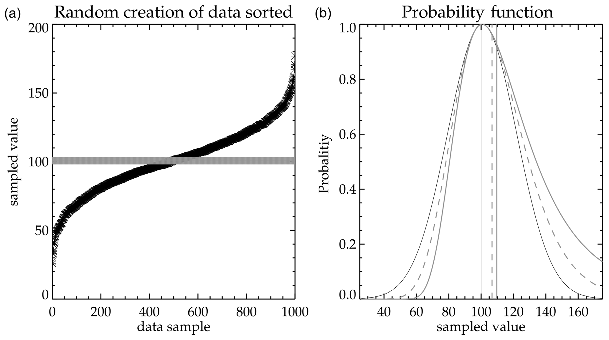
Figure 3 This shows how a randomly sampled measurement within a volume would compare to a whole sample volume-averaged measurement. The left panel shows randomly generated measurements based on a Gaussian distribution having a mean value of 100 with a standard deviation of 25. The + symbols represent the individually generated measurements (as measured in situ) that make up an average value of 100 (as measured remotely). Panel (a) shows the probability of measuring a particular difference based on how that difference is computed. Thin black is y−x, thick gray is $(y-x)/x$, and thick dashed gray is $\mathrm{2}(y-x)/(x+y)$. The vertical lines are their means.

Figure 4 shows a coincident humidity comparison between AIRS and the Earth Science Research Laboratory (ESRL) BFH that is routinely launched from Boulder on a monthly basis. The comparison pressure is 261 hPa. Next to it is a comparison between MLS and the BFH at 100 hPa. Averaging kernels were not applied to either data. The BFH data have been sorted by value and show a similar shape to those in Fig. 3. Likewise, both AIRS and MLS show a generally flatter response. In addition to the spatial-averaging variation, there is atmospheric variability that accounts for why the slope for the satellite measurement is not zero like it is in the demonstration plot (Fig. 3). Additionally, satellite spatial averaging and the retrieval itself over the sampled volume will exhibit some nonlinearities and non-Gaussian behavior. Therefore, while a comparison like that in Fig. 3 may not look good, the reality is that the agreement may actually be as good as one can expect because of the very different characteristics of the measurements themselves. It is also important to recognize that the dynamic range of measurements at 261 hPa is 10–400 ppmv versus the stratospheric 100 hPa which runs from 2.5–7.5 ppmv. The smaller dynamic range for the stratospheric measurements suggests that H₂O is more tightly regulated by large-scale atmospheric processes (e.g., tropical tropopause temperature, transport, and chemistry). This is shown in the MLS-Aura comparison which generally tracks the BFH values even through to the highest values. However, MLS-Aura appears to overestimate the extreme lower values. BFH versus MLS-Aura and the MIPAS suite comparisons at 261 hPa look similar to those shown for AIRS and, at 100 hPa for the MIPAS suite, look similar to those shown for MLS-Aura.

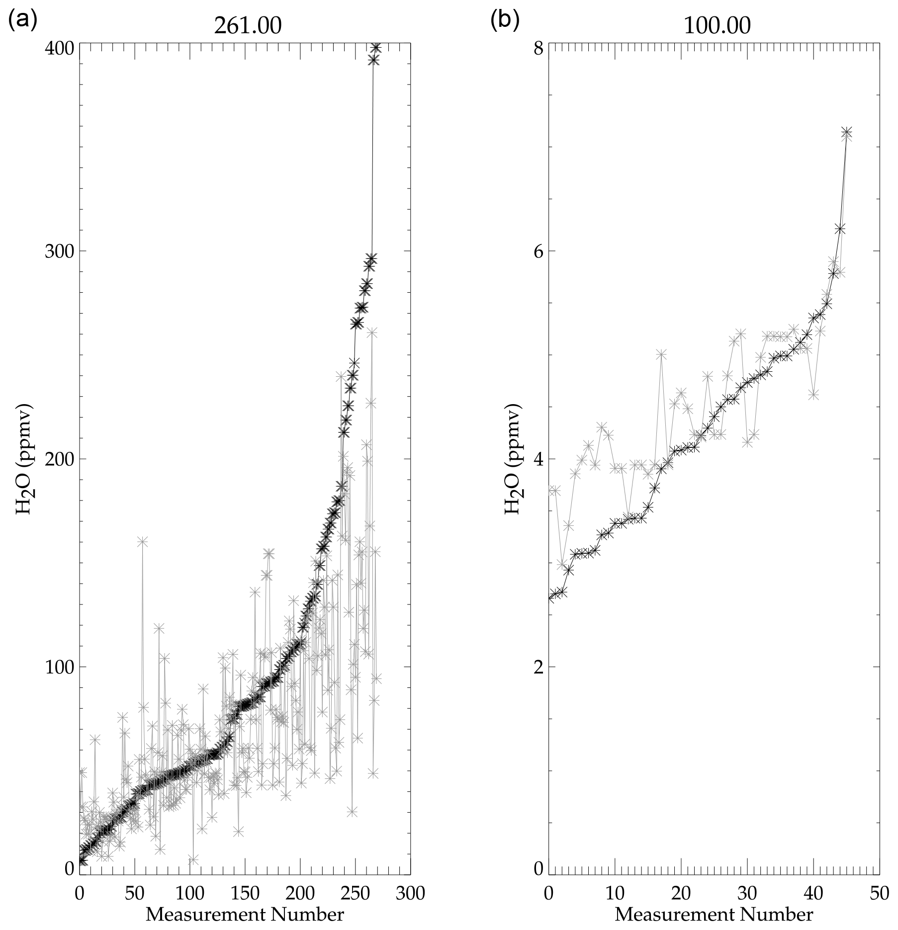
Figure 4 A comparison of coincident Boulder BFH and AIRS measurements (a) at 261 hPa and MLS-Aura measurements (b) at 100 hPa is shown. The BFH measurements are sorted by value, black, the satellite measurements in gray.

5 Coincident comparisons

5.1 Balloon frost-point hygrometers

Figure 5 summarizes results of coincident comparisons between BFHs launched from Boulder and some individual satellite data sets with and without application of the averaging kernel. The averaging kernel is applied (Livesey et al., 2020) to the coincident sonde profiles for the MIPAS and MLS data set. Although applying the averaging kernel to a highly vertically resolved measurement when comparing to a remote sensing measurement is the proper method for comparison, in practice there are some limitations. These include neglect of nonlinear forward model effects (causes the averaging kernel function to be profile shape and amount dependent) and truncation effects when the balloon does not achieve high altitude. For some of the retrievals, applying the averaging kernel makes the agreement worse, in particular the MIPAS-Oxford retrieval. It is not understood why applying averaging kernels to the data for this particular data set should have made the agreement worse, but the averaging kernel function does depend on the profile shape and concentration. Each data set producer provided representative kernels to use with their data set, and perhaps those for the Oxford data were a poor match for the profiles shown here. For MLS-Aura, which has the highest number of coincidences, applying the averaging kernel makes very little difference. The same is also true of the MIPAS-IMK retrieval. Offline simulation studies done on MLS support the above result. The averaging kernel is important for the 121 hPa and lower-pressure levels (i.e., higher in altitude) but was not important for the higher-pressure levels (i.e., lower in altitude) (Read et al., 2008). Averaging kernels are not available for all the data sets used here, e.g., AIRS. Therefore, there is no advantage to be gained from using the averaging kernel, and for consistency in handling of the data sets here it is not used in the following analysis.

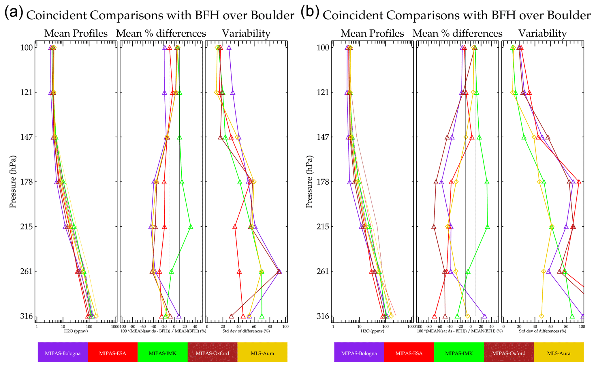
Figure 5 Summaries of coincident profile comparisons between Boulder BFH without averaging kernel applied (a) and with averaging kernel applied (b) as well as the satellite data sets. The data sets are color coded according to the caption below. The leftmost in the group of three panels shows the mean of the coincident profiles (thick with symbols) for the satellite data set and the corresponding mean for the BFH (thin line). The center panel within the triad shows the mean bias, and the right panel within the triad is the variability about the mean.

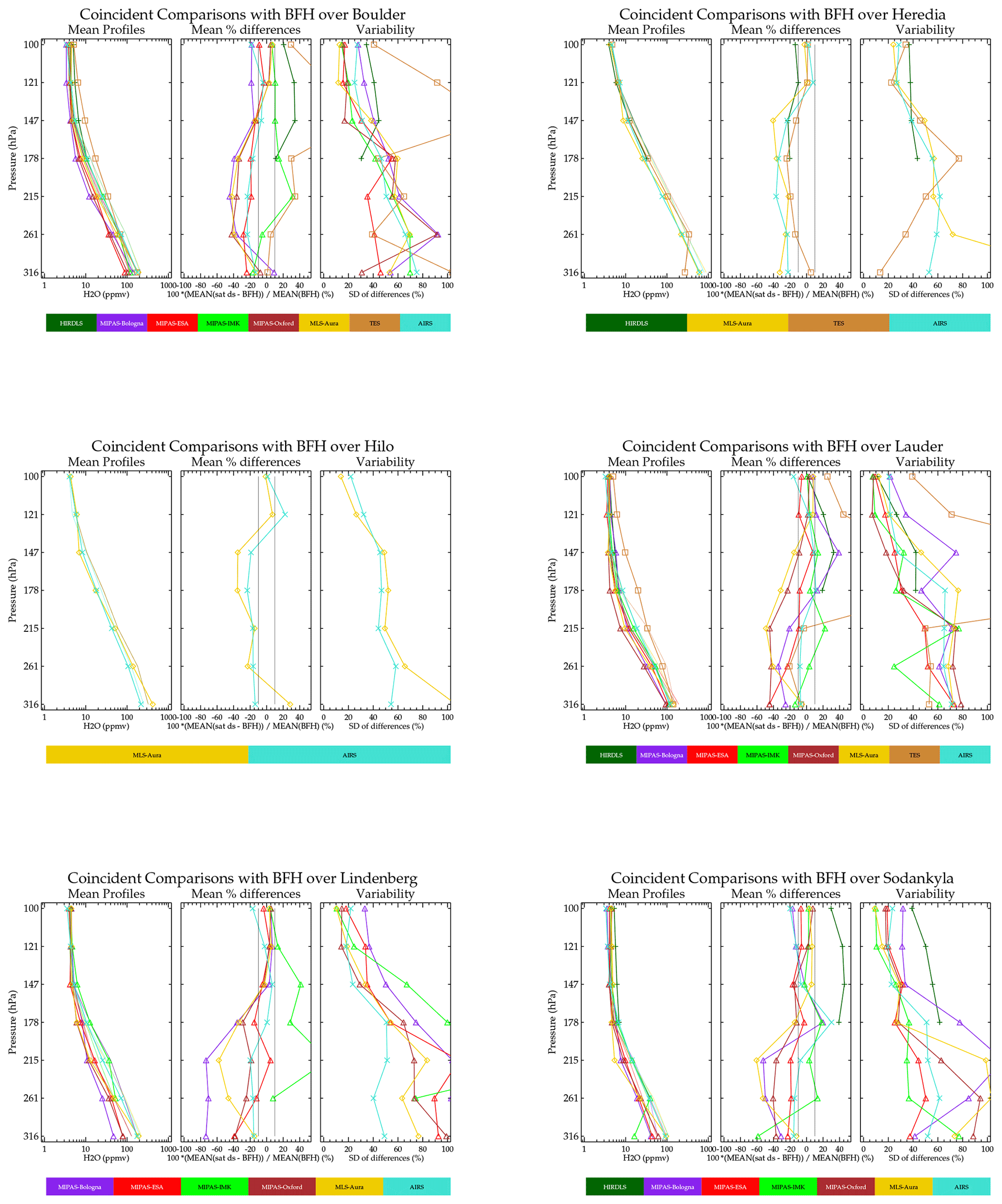
Figure 6 is a summary of coincident scatter plot comparisons between BFH and satellite retrievals where there are enough coincidences to generate some statistics (seven or more). The tight coincidence matching criterion limits these comparisons to passive limb sounders. For each sonde site, the left panels show the mean profile of the coincidences being measured. The thick lines with symbols are the satellite data sets, and the lines without symbols represent the mean of the coincident sonde profiles. Since the actual coincidences differ in number and time of measurement, the means of the sonde profiles will be different for each instrument. The center panel shows the bias in percent. The right panel shows the variability of the coincident differences about the mean difference. The root mean square of the coincidently compared profiles is the square root of the sum of the bias (center panel) squared and the variability (right panel) squared.

The comparisons in Fig. 6 show mean coincident agreement within several tens of percent of the BFH with a scatter about the mean value of 20 %–60 % for most instruments. AIRS shows the best agreement overall. MIPAS-IMK shows typically 20 % agreement but with a positive bias. The other MIPAS retrievals (Bologna, ESA, and Oxford) are mostly drier. MLS-Aura is also drier but consistently shows a significant dry bias for the level that is 2–3 km below the tropopause. For the mid-to-high latitudes, this is near 215 hPa, and for the tropical latitudes it is at 147 hPa. Curiously, the MIPAS-Bologna retrieval also exhibits this behavior for the midlatitude comparisons, but it is not possible to determine if this is linked to the tropopause height as there were no suitable comparisons in the tropics. HIRDLS shows moist biases for the midlatitude sites but a small dry bias at the Heredia (tropical) site.

Figure 6 Same as Fig. 5 but for different BFH locations. No averaging kernel was applied.

5.2 Time series comparisons

Another way to look at the humidity data is through a time series. This type of comparison shows how each satellite data set will capture seasonal cycles and interannual variability. Comparisons are shown in two formats. Figure 7 shows an overlay of BFH sonde measurements at Boulder with smoothed reconstruction of satellite measurements in the vicinity of Boulder (±2.5^∘ longitude and latitude). Temporal coincidence with the actual Boulder sonde launches is not imposed. As is shown in the figure, most of the data sets capture similar annual cycles with varying degrees of fidelity relative to the sonde. Interannual variability is similar among the majority of the data sets and sonde. For example, 2007 shows higher values and a stronger seasonal amplitude than during the succeeding 2 years.

Figure 7 Time series of BFH and satellite and retrievals having enough data coincident with Boulder to produce a smoothed time series curve. The BFH data show the individual measurements in addition to the smoothed curve. Only smoothed curves are shown for the data sets to remove excessive data clutter.

Figure 8 shows the time series over Hilo (Hawaii), a tropical site. As with Boulder, most of the satellite retrievals capture the seasonal cycles seen in the BFH sonde data. One exception is MLS-Aura at 147 hPa, which shows a much weaker amplitude than the BFH sonde and is also drier (MLS-Aura is not unique in this respect though). This feature was noted in a comparison report by Hegglin et al. (2013). The explanation for this relates to the tropopause height dependence of the dry bias seen in the MLS-Aura sonde comparisons. Over the tropical sites, the tropopause is rising and falling by ∼1.5 km over the year; thus, the MLS-Aura bias also rises and falls with it causing a potential flattening of the annual cycle. Notice in Fig. 6 that the bias gradient with the tropopause height is rather steep. The midlatitude locations where the tropopause is near 147 hPa shows a 50 %–60 % dry bias for MLS-Aura at 215 hPa and much smaller 10 % dry bias at 147 hPa. For the tropical sites, where the tropopause is near 100 hPa, the dry bias at 215 hPa drops to 10 %–15 % but increases to 40 % at 147 hPa. Therefore, a seasonally modulating tropopause height would be expected to modulate the MLS dry bias significantly for the level that is 2–3 km below the tropopause or in this case the 147 hPa level, as well as the levels above and below but to a lesser extent. Subsequent investigation of this bias suggests that it is caused by a pointing difference error between the radiometer that measures water vapor and the radiometer that measures O₂ for pointing. This bias is corrected in version 5 (Livesey et al., 2022). Version 5 shows that the pointing error in v4 does flatten the 147 hPa annual cycle (in contrast to accentuating it).

Figure 8 Same as Fig. 7 but for Hilo, Hawaii.

Figure 9 shows a data-smoothed time series comparison over Sodankylä, Finland, which is a high-latitude Northern Hemisphere site. The BFH shows a weak annual cycle at 147 hPa and stronger ones at lower altitudes. This behavior is captured by most of the data sets.

Figure 9 Same as Fig. 7 but for Sodankylä, Finland.

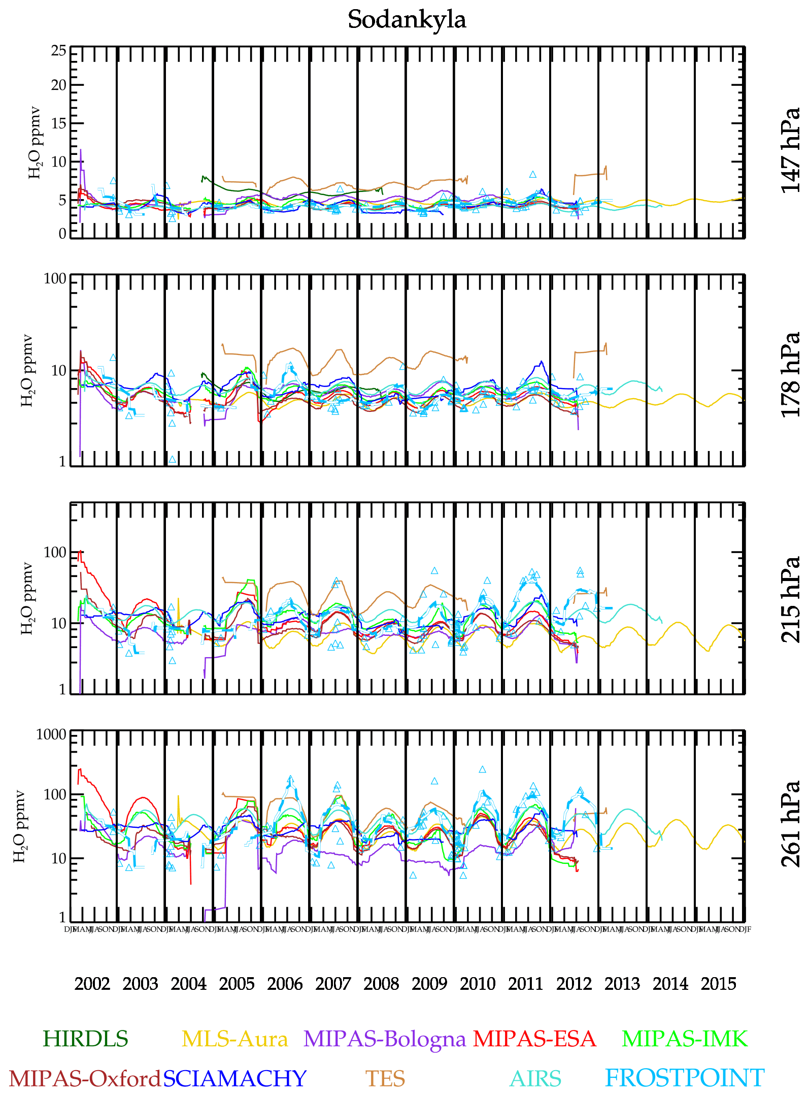
Figure 10 shows a data-smoothed time series comparison over Lauder, New Zealand, which is a midlatitude Southern Hemisphere site. The BFH shows an irregular seasonal cycle that in most years is weak at 147 hPa except at the beginning of 2007. Most satellite measurements show larger seasonal cycles with a more regular phasing. The phasing does differ among the satellites.

Figure 10 Same as Fig. 7 but for Lauder, New Zealand.

Exploring the question of seasonal amplitudes and phase further, the time series data are fitted to a periodic function that yields a mean value, annual cycle amplitude, and phase. Interannual variability is ignored in this fit; thus, the result should be viewed as a “climatology”. The result for Boulder, USA, is shown in Fig. 11. The data sets capture the annual cycle with correct phase. Figure 12 shows a comparison of the fitted function to Hilo data. It is noteworthy that MLS-Aura greatly underestimates the seasonal cycle at 147 hPa relative to the other data sets and BFH sondes. This feature is present regardless of whether averaging kernels are applied or not, and its cause has been identified.

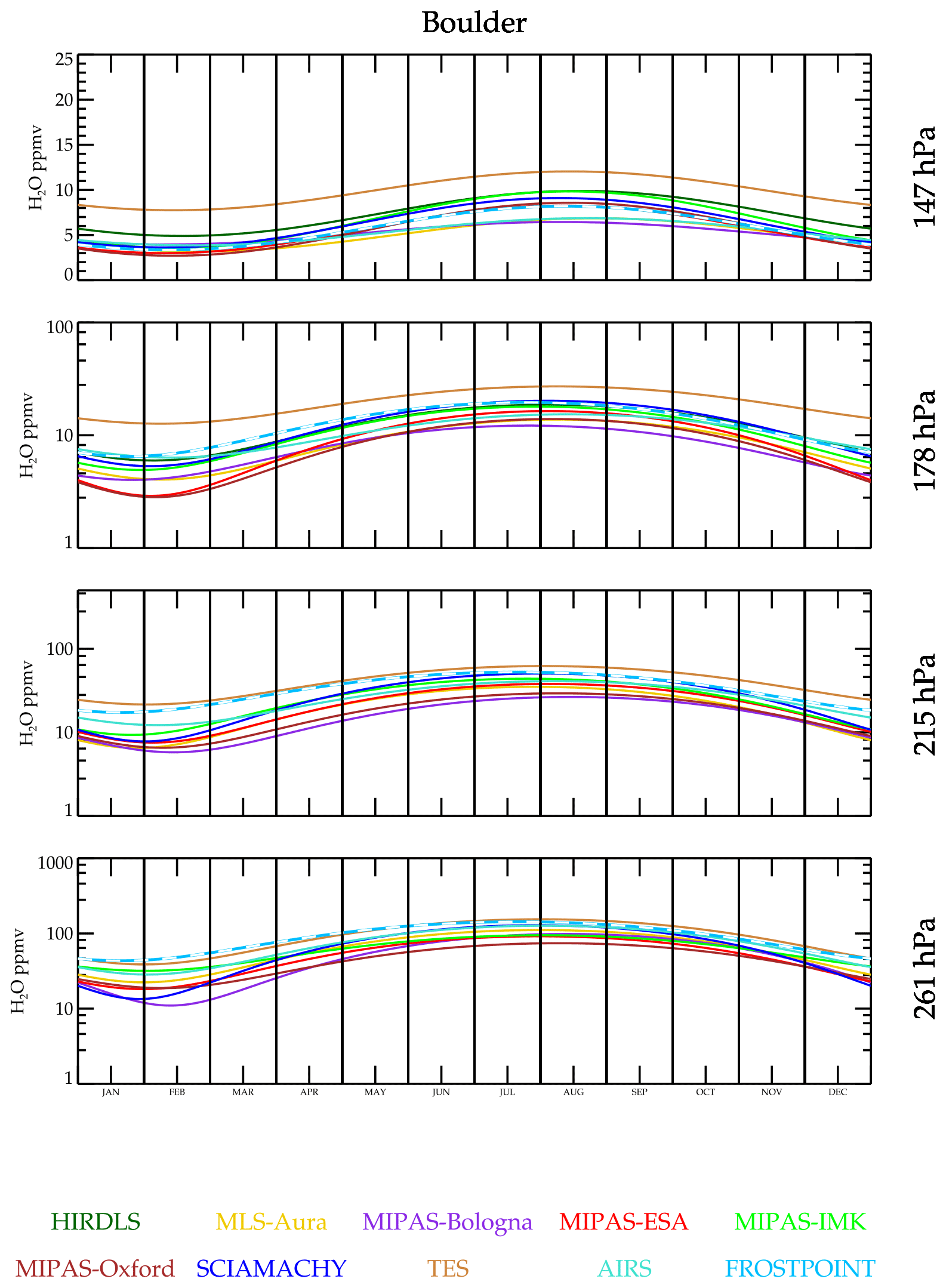
Figure 11 For each data set, a periodic 1-year function is fitted to the time series data near Boulder, CO, and plotted for 1 year. Interannual variability is averaged over for each data set. Therefore, this figure is a climatology for that data set.

Figure 12 Same as Fig. 9 but for Hilo, Hawaii.

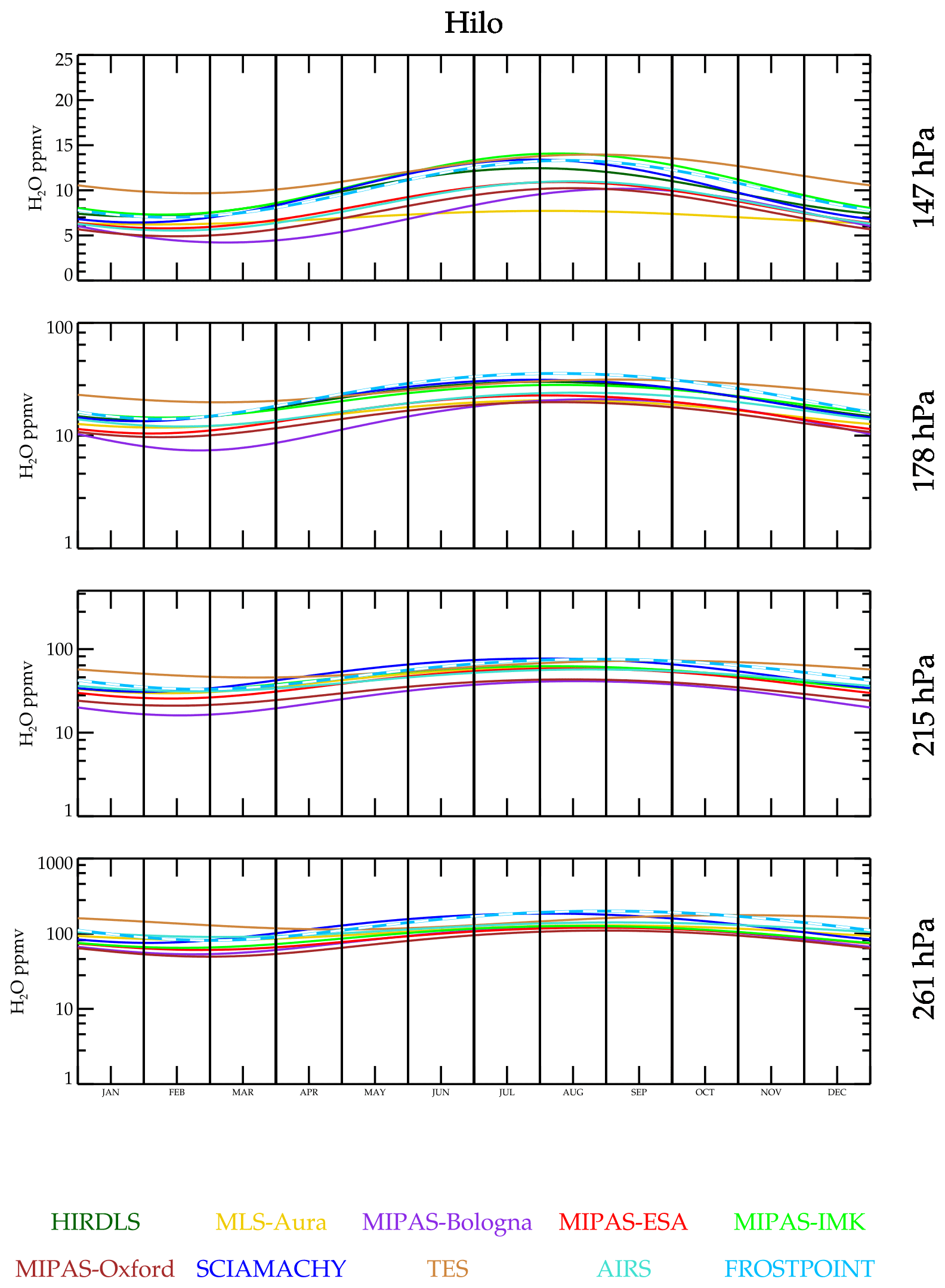
Figure 13 summarizes the results from fitting a periodic function to the coincident data for the six sonde sites. Ideally, the left panels in Fig. 13 should be similar to the center panel in Fig. 6. The difference between these is that Fig. 6 is based on location and temporal coincidences, whereas Fig. 13 is based only on location coincidences and uses a function to interpolate in time. While the former is the better method of comparison, because of the limited number of sonde launches, statistics are sparse, and very few instruments can be compared. The fitted time series function approach improves the statistics, and a few more instruments can be compared; however, differences in temporal sampling impact the comparison. At Sodankylä, the seasonal cycle at 147 hPa is weak, and no instrument captures it well based on the BFH time series fit. Most instruments do much better at the lower altitudes. Over the two tropical sites as noted before, MLS-Aura significantly underestimates the annual cycle amplitude. SMR underestimates the annual cycle at all four altitudes shown here. BFHs launched from Lauder also have a weak seasonal cycle at 147 hPa. Most of the satellite instruments, including MLS-Aura, tend to overestimate the seasonal cycle relative to the BFH. Also, the phasing in the BFH is irregular, and the fit is dominated by the large moist event that occurred in late 2006 and early 2007.

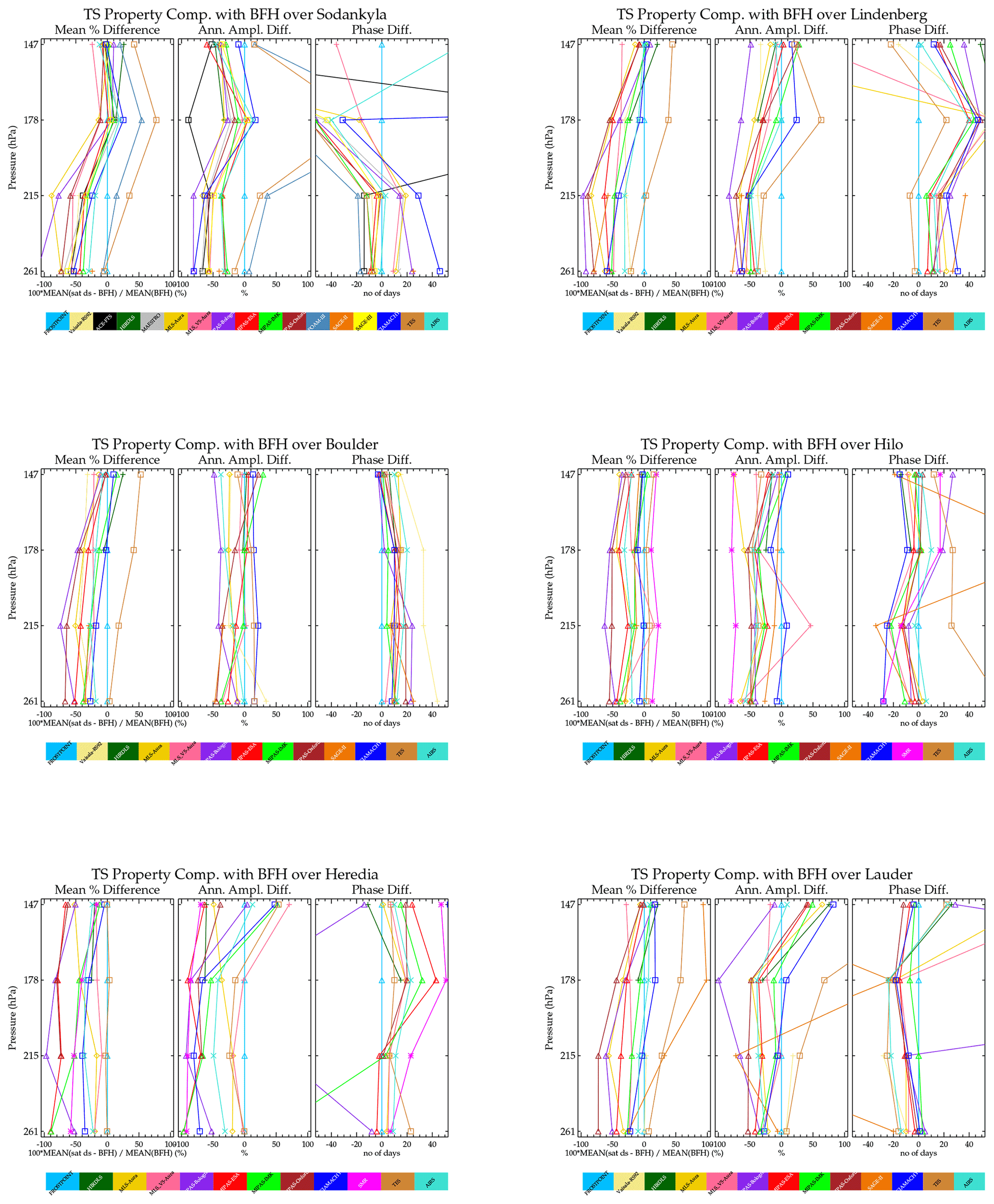
Figure 13 Comparisons of fitted periodic function parameters (mean value, left; amplitude, center; and phase, right) between a data set (colored line) and BFH sonde as a function of altitude (pressure).

Figure 14 shows mean biases between BFH and instrument data sets derived from mean differences of spatial and temporal coincidences and mean value derived from fitting to all data with a periodic function that is only spatially coincident. AIRS and MLS-Aura, the data sets with the best statistics for the coincident comparisons, show the best agreement for a mean derived from a time series fit and a mean from a coincident comparison fit. Even for these data sets, the agreement between the two methods is as large as 20 %. The lack of consistency between sonde values and the direct coincidences prompts us not to use derived biases as a proxy for direct coincidences when summarizing results later in this paper.

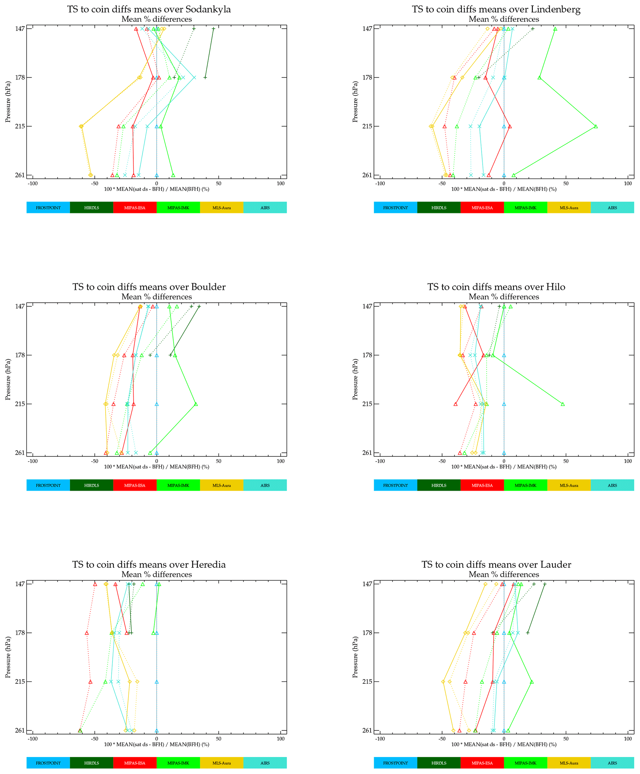
Figure 14 Comparisons of biases computed from direct location and temporal coincidences (solid lines) versus that derived from a time series function using all available data satisfying a positional coincidence criteria (dotted).

Figures 15 and 16 show time series and scatter plot comparisons of satellite measurements with Vaisala RS92 balloon hygrometers over Southern Great Plains, USA, and Sodankylä, Finland. The Vaisala RS92 sonde uses a capacitance hygrometer that is precalibrated by the manufacturer prior to launch. These hygrometers are relatively inexpensive and therefore launched more often than BFH. Unfortunately, these capacitive hygrometers are not accurate near the tropopause nor in the stratosphere. The response time of the capacitive element lengthens as the humidity approaches stratospheric concentrations and thus become erroneous under extremely dry conditions. Postprocessing algorithms have been developed to compensate for this time lag and correct these data based on coincident BFH launches during campaigns (Dirksen et al., 2014). Comparisons here indicate that the Vaisala RS92 instruments, even with corrections, are probably not reliable for concentrations <10 ppmv. Figure 15, showing a comparison over the Southern Great Plains region of the USA, shows reasonable correlations at all levels including 147 hPa. The time series measurements show that during Northern Hemisphere summer, very high values (∼20 ppmv) are often prevalent. It has been shown that summertime deep convection can indeed inject high amounts of H₂O into the stratosphere (Anderson et al., 2012; Schwartz et al., 2013), which is consistent with the concentrations shown here. Therefore, one might conclude that the RS92 with the correction algorithm is successful. But caution is definitely in order here. Launches over Sodankylä (Fig. 16) present a different view. Like the Southern Great Plains site, the RS92 shows a prevalence of very high humidity events occurring during the Northern Hemisphere summer that are not seen in any satellite data set. A scatter plot with MLS-Aura is shown as it had the most coincidences, but all the MIPAS retrievals are identical in that there are no high humidity events (>10 ppmv) seen over Sodankylä at 147 hPa. The dashed lines are an orthogonal distance regression fit to the scatter points. When both the x and y data sets have large and unknown error, and orthogonal distance regression is a reasonable method for determining the correlation. In the case for the 178 and 147 hPa at Sodankylä, the correlation is so poor that a best-fit line is meaningless; therefore, it is omitted for clarity. The correlation at 178 hPa is also poor, again with the Vaisala RS92 showing extremely dry and moist events, whereas the satellites have measurements usually between 3–8 ppmv. Other sites with frequent launches, including Lindenberg, Germany; Ny-Ålesund, Norway; Barrow, USA; Cabauw, the Netherlands; and Lauder, New Zealand, behave like Sodankylä. It probably should be assumed that the highest-altitude pressure level for which the RS92 can be used is ∼200 hPa with humidity concentrations exceeding 10 ppmv. It is likely that some of the high values measured by RS92 over the Southern Great Plains are accurate measurements as the capacitance sensor responds best to more moist conditions, but given that equally high values are seen elsewhere where they are unlikely to be present makes such measurements suspect. A case in point is Lindenberg where there were a high number of both BFH and RS92 launches. At 147 hPa, neither the satellite sensors nor the BFH show a measurement exceeding 10 ppmv, whereas the RS92 instrument shows a large number of them. For pressures greater than 200 hPa, compared to coincident BFH instrument that fly together, the RS92 has a 10 % dry bias with a 20 % standard deviation.

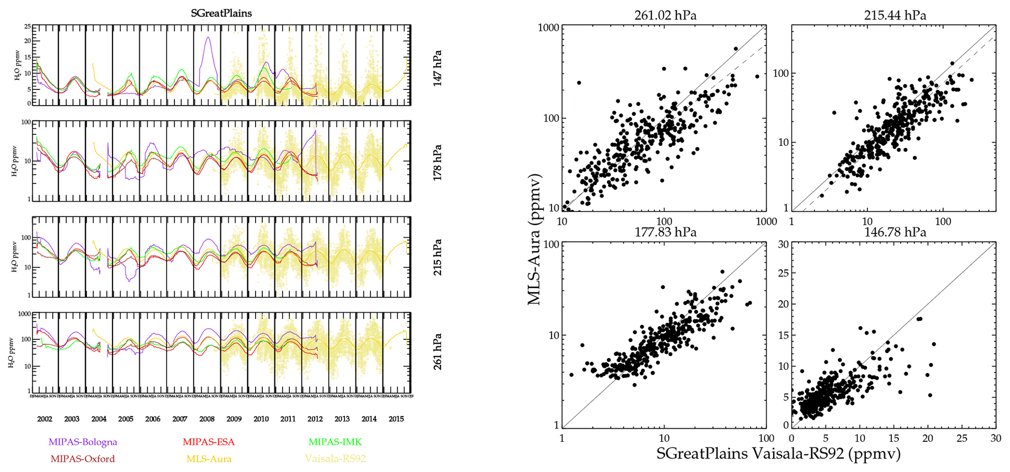
Figure 15 Smoothed time series (left) and scatter plot (right) comparing Vaisala RS92 hygrometer versus satellite instrument and retrievals at Southern Great Plains, USA.

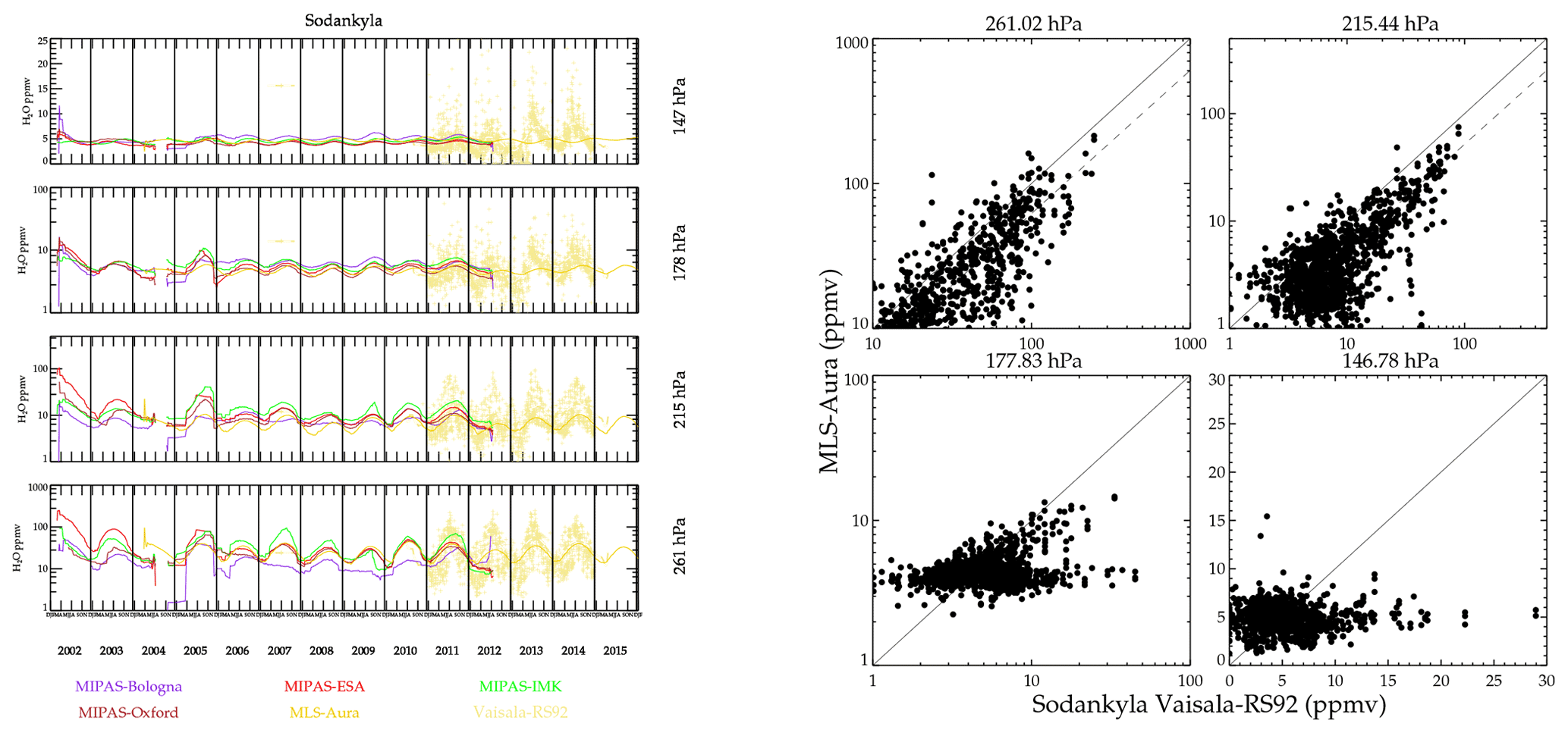
Figure 16 Smoothed time series (left) and scatter plot (right) comparing Vaisala RS92 hygrometer versus satellite instrument and retrievals at Sodankylä, Finland.

5.3 Satellite-to-satellite coincident comparisons

Coincidences between satellite data sets are discussed here. Figure 17 shows a coincident match scatter plot comparison between MLS-Aura and ACE-FTS as a probability density function (PDF). Only data below the MERRA-5.2 tropopause height are considered. In order to get some coincidences, the time match is expanded to 18 h. Without this, there would be no coincidences except at the highest latitudes where MLS-Aura, in a sun-synchronous orbit, samples local times encompassing the sunrise and sunset, i.e., the times sampled by occultation. A relative density amount for each contour is shown in the color bar. Since the number of coincidences decreases with altitude, only data below the tropopause are being compared; the scale is relative. The number in all bins is divided by the number in the bin having the greatest number of points and assigned a color. The solid circles on the thick line define the bins whose H₂O concentrations are values shown on the x axis. The bin values for the y data set are the same as those on the x data set. The thin line is the mean value of the y points within the x bin, the thick line is the corresponding median value, and the dashed lines are 1σ standard deviation about the mean value. As can be seen in the plots, ACE-FTS is usually more moist than MLS-Aura.

Figure 18 shows a comparison between MLS-Aura and MIPAS-IMK. Note that there are essentially no coincidences in the tropics due to the 3 h coincidence criterion (the Equator-crossing local solar time (LST) for Aura is 13:45 LST versus 10:00 LST for ENVISAT). As with ACE-FTS, MLS-Aura tends to be drier. Figure 19 shows a scatter comparison between MIPAS-ESA versus MIPAS-IMK. Since these are different retrievals from the same instrument, all measurements are coincident, and all latitudes are covered. This shows that MIPAS-IMK is more humid than the ESA product. One thing that is noteworthy in all these plots is the stretched S-shaped curve of the means and medians. The lowest x bins have y values that are more moist, and the highest x bins have drier y values. This feature persists even if the x and y instruments are interchanged. The extreme x-axis value bins are populated with few values and are probably poor retrievals not caught by screening criteria. The corresponding y values are probably better measurements and more accurately represent the atmospheric state. Many plots of this type were generated and are deferred to in the Supplement. The summary of the results is presented in Sect. 7.

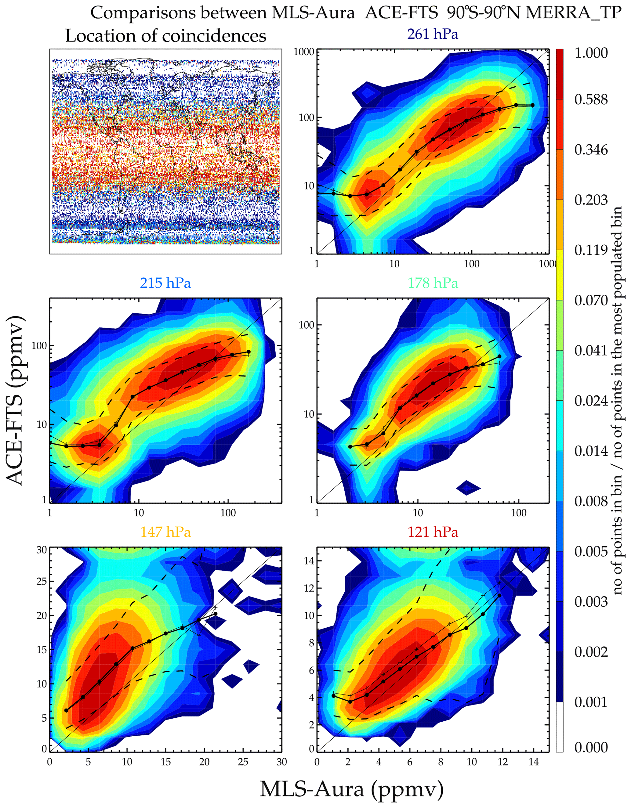
Figure 17 Contour probability density function (PDF) plots of coincident humidity measurements between MLS-Aura and ACE-FTS. Only data below the tropopause are shown. The top left panel shows the location of the coincidences, and the points are color coded by the pressure level closest to but below the tropopause height. The color bar shows the ratio of points in an x–y concentration bin to bin with the maximum number of points. The coincidences cover a period from August 2004 to March 2019.

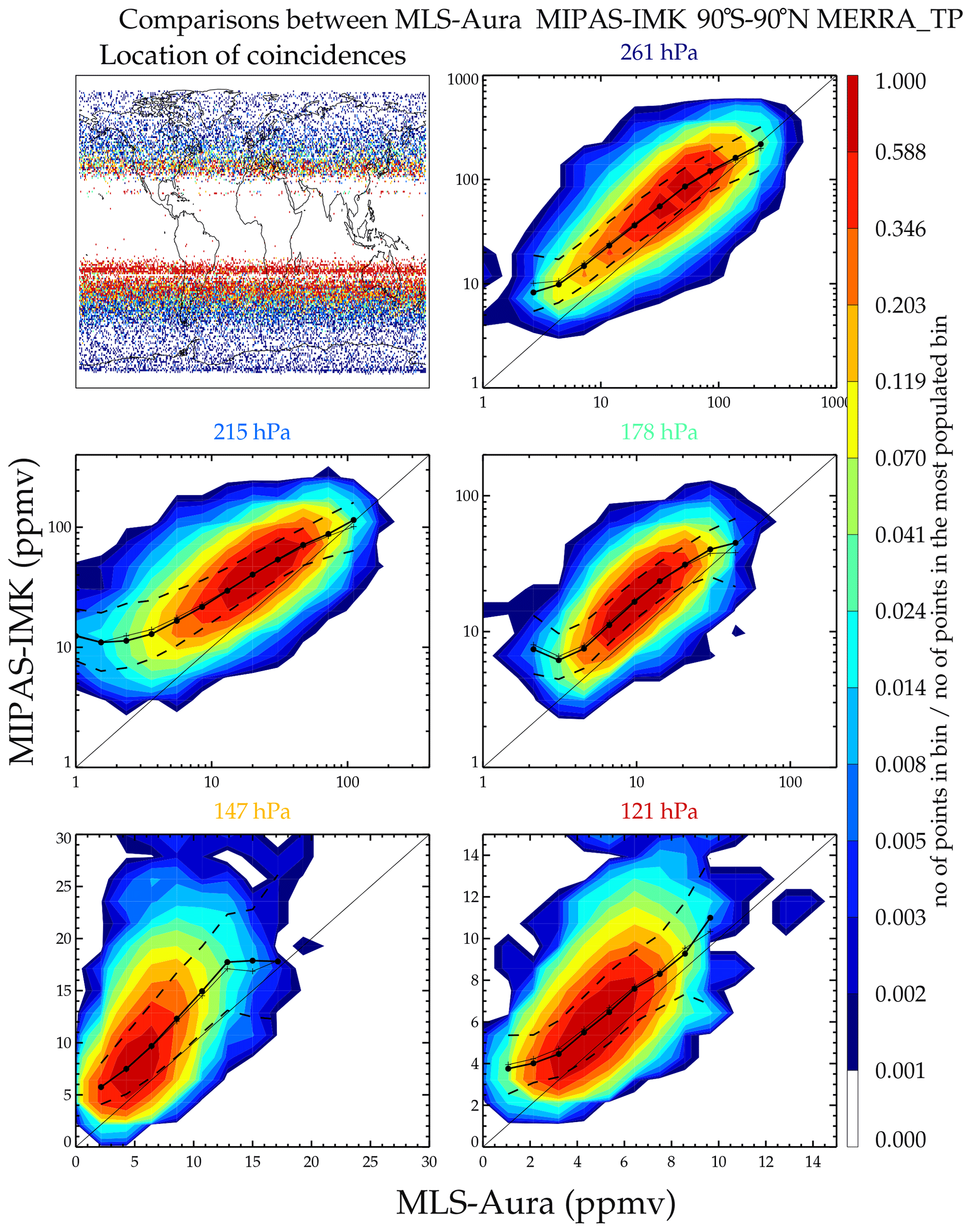
Figure 18 Same as Fig. 17 but comparing MLS-Aura and MIPAS-IMK. The coincidences cover a period from January 2005 to April 2012.

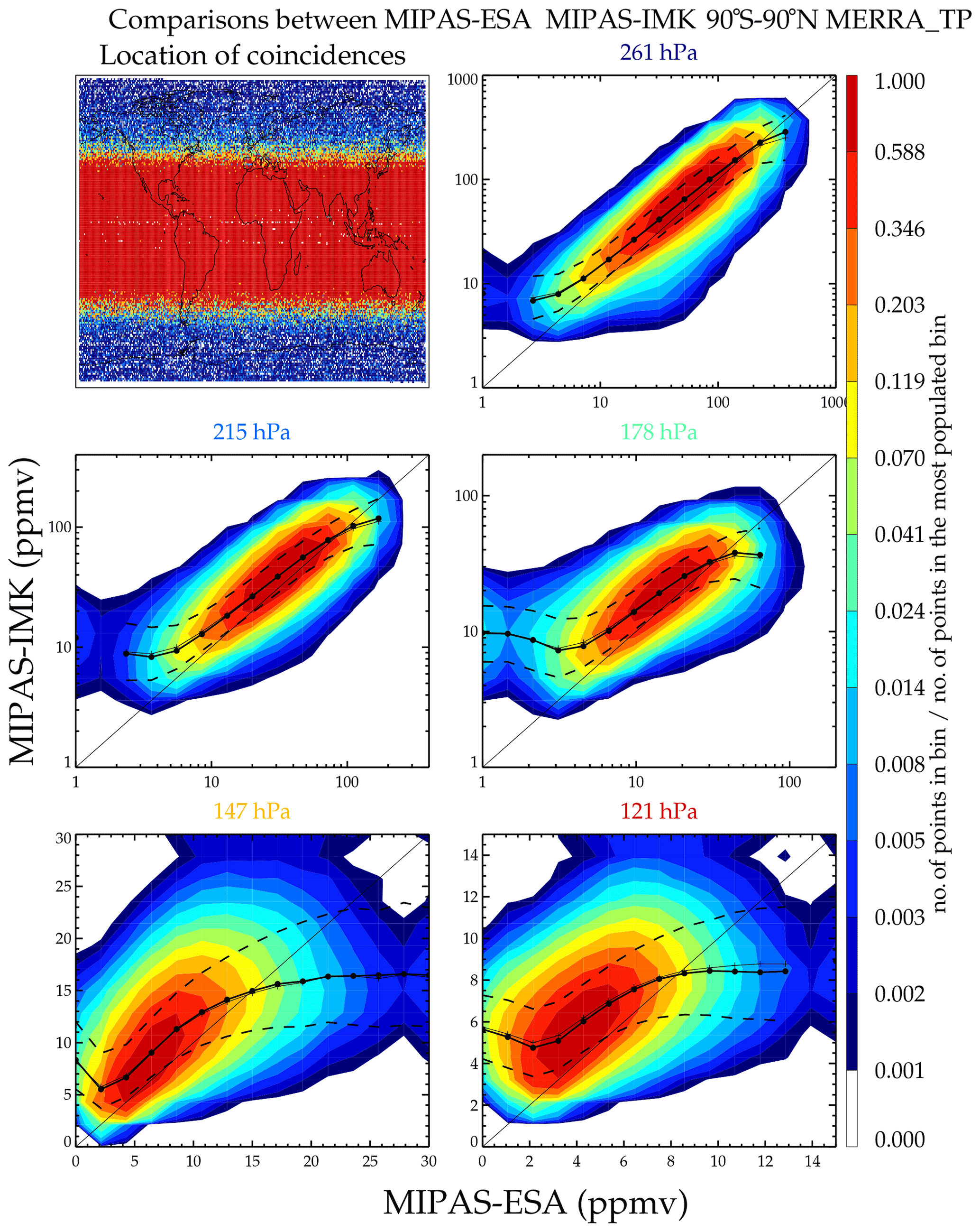
Figure 19 Same as Fig. 17 but comparing MIPAS-ESA and MIPAS-IMK. The coincidences cover a period from July 2002 to April 2012.

5.4 Gridded map comparisons

Gridded map comparison is another method where climatologies can be compared. It has the advantage of not requiring coincidences, and inter-measurement coincident matched variability should average down as each grid box represents an average over several measurements. Therefore, variability that would be seen when comparing individual coincident differences averages down, revealing mostly a bias if there are enough values sampled. Its weakness is that sampling biases can significantly affect the comparison. The pressure levels used for these comparisons use the AIRS level-3 gridded product standard levels (300, 250, 200, 150 hPa). AIRS has the best global sampling and therefore produces statistically the best coverage. This decision avoids having to vertically interpolate two data sets simultaneously (e.g., AIRS and MIPAS, for example, to an MLS standard pressure level such as 178 hPa). Figure 20 shows 3-month gridded maps of AIRS and MLS-Aura for June 2012–August 2012. The gridding resolution is 5^∘ longitude and 4^∘ latitude in Fig. 20. This period is shown to highlight a time where MLS-Aura underestimates humidity at 147 hPa over Costa Rica and Hilo, Hawaii (Fig. 8). The morphological agreement is excellent. The quantitative agreement will be shown in detail later and is mostly good. An exception here in particular is the contrast between Central America versus Asia at 150 hPa. Although both instruments show that these are moisture-rich regions, MLS-Aura shows a much greater moisture difference between Asia and Central America than AIRS does. Based on two tropical BFH sondes sites, MLS-Aura should have a larger dry bias at 150 hPa than AIRS, and the mapped field over Central America is consistent with this; however, this behavior does not extend throughout the tropics as MLS is considerably more moist than AIRS over Asia. In contrast, 300 and 250 hPa fields show MLS-Aura being more humid than AIRS over Central America and Asia.

AIRS is a downward-looking instrument that views nine 15 km infrared scenes. The nine scenes are combined together to estimate each scene's cloudiness and produce a clear-sky radiance signal that is assumed to be homogeneous over the 45 km scene (Susskind et al., 2003). The clear-sky scene brightness can be shown to be proportional to the logarithm of the relative humidity divided by the atmospheric temperature gradient (Soden and Bretherton, 1993). Vertical sampling and thus resolvability is achieved by spectrally resolving the signal. The H₂O absorption line shape causes the emitting signal to become opaque at different altitudes in the atmosphere, and due to the temperature gradient in the atmosphere, a spectral signal is observed that allows a vertically resolved measurement to be made. MLS is a limb-viewing instrument whose FOV (field of view) is scanned across the Earth's limb. MLS also resolves a spectrum that varies with scan. The H₂O absorption line shape also produces an emission line shape that varies in width due to pressure broadening; however, unlike the downward-looking viewing instrument, its thermal background is cosmic (2.7 K) and does not require the atmospheric temperature to have any special property except to be warmer than the cosmic background. The limb-viewing geometry has a much longer path length in the atmosphere than a downward-looking view does. This allows very small concentrations to be measured with great precision, but there is an upper limit to the maximum measurable concentration (typically 1000 ppmv) that restricts this technique to the upper troposphere. Another issue is that the long atmospheric path length almost ensures that cloud contamination is present. MLS manages to avoid this problem by using long wavelengths that are largely invisible to clouds except under severely convective environments. There is a simplified mathematical description of radiances seen by the limb-viewing and downward-looking geometries presented in Read et al. (2007).

The fields track the tropopause well where the values become stratospheric like (<10 ppmv) poleward of the tropopause contour. Tropopause tracking is generally better with MLS than AIRS, because the limb-viewing technique does not require an atmospheric thermal gradient to provide spectral contrast in the measurement and MLS most likely has better vertical resolution across the tropopause. Quantitatively, MLS at all levels tends to show higher humidity at the extreme wet regions and more dryness in the desiccated regions than AIRS except over Central America at 150 hPa. These kinds of plots have been made for other months and years, and the characteristics of the comparisons are the same despite changing morphologies.

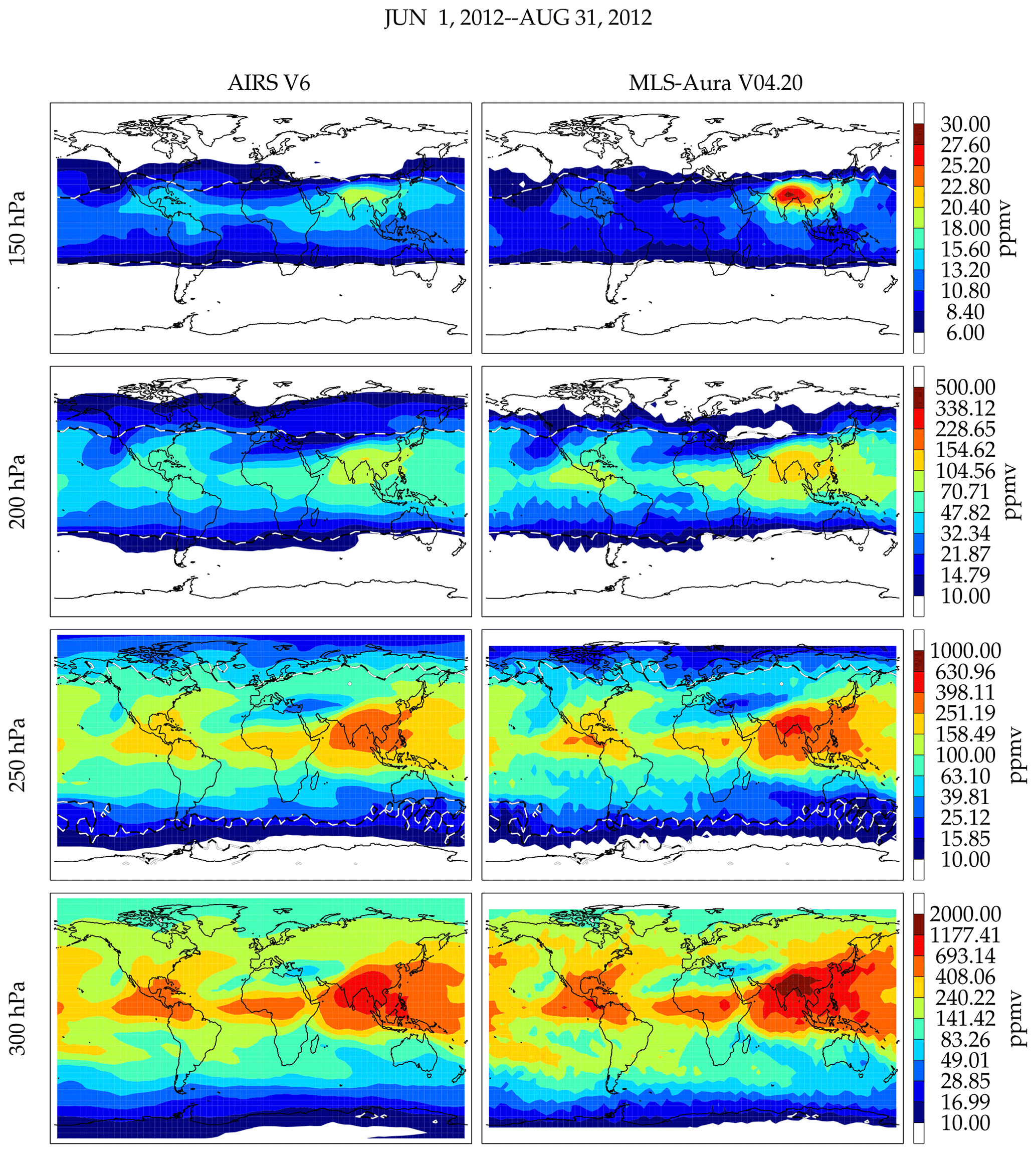
Figure 20 Gridded map comparison between MLS-Aura and AIRS V6 during June–August 2012. The tropopause is indicated by the black and white dashed contour line. Equatorward of this line is in the troposphere and poleward of this line is in the stratosphere. The white regions are H₂O<10 ppmv. MLS has no measurements poleward of 82^∘.

Figure 21 shows a scatter plot of the gridded map values between AIRS and MLS-Aura. The scatter plot provides a more quantitative assessment of the gridded values than can be seen from comparing contour plots. The correlation is good; however, the slopes of the correlations are greater than one, because MLS-Aura tends to exaggerate the extreme moist and dry values relative to AIRS. The Asian moist bias in the MLS-Aura measurement is evident in the 150 hPa panel.

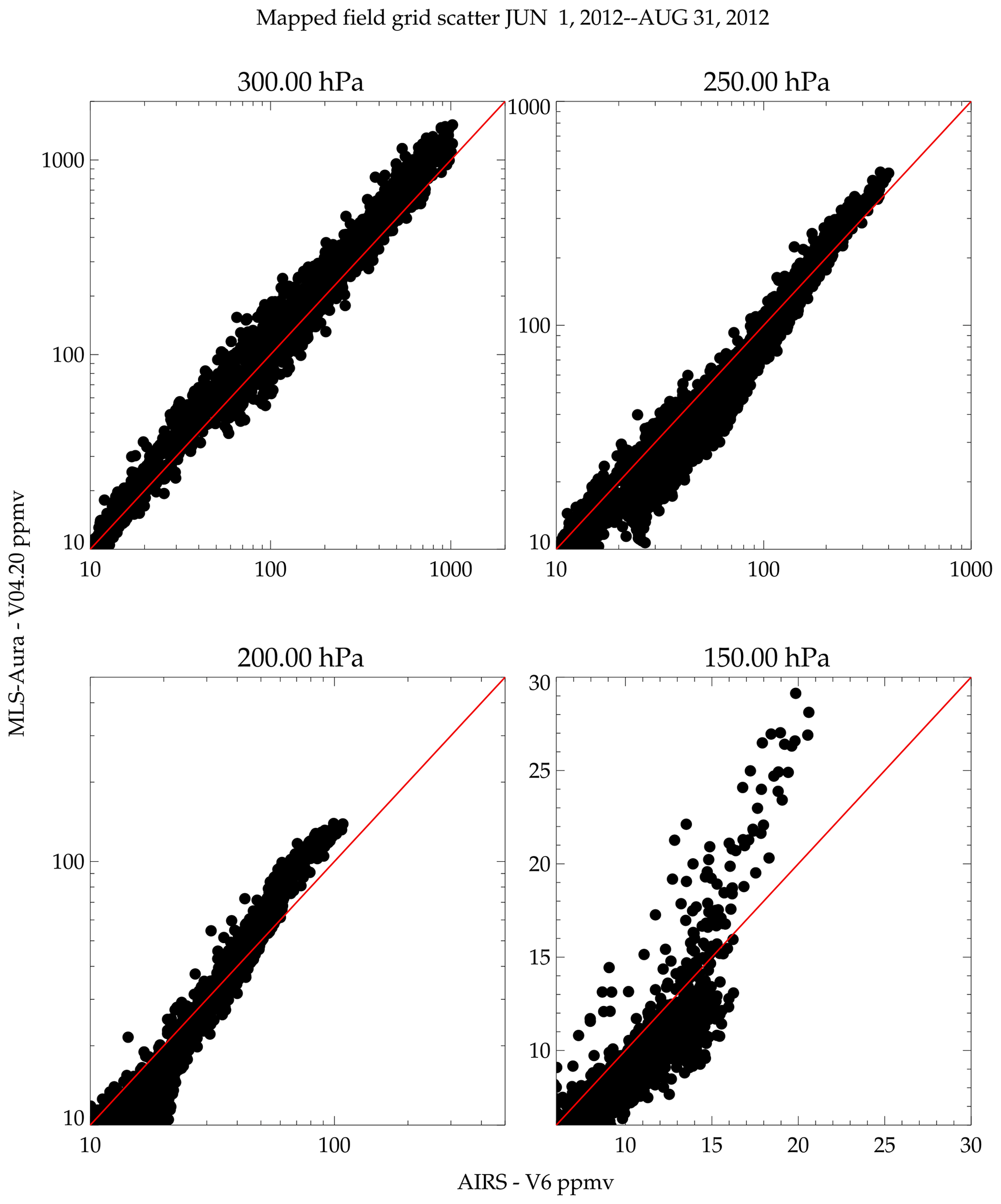
Figure 21 Scatter plot comparison of the gridded box values in Fig. 20 between AIRS and MLS-Aura during June–August 2012. The red line is the one-to-one line.

Figure 22 shows humidity maps at 175 hPa from nine other data sets. HIRDLS, MLS-Aura, MIPAS, and SCIAMACHY are limb-viewing instruments, whereas SMR (in UTH retrieval mode) and TES are downward-viewing instruments. These data sets sample the Earth less frequently than either AIRS or MLS: the grid box size is 10^∘ longitude by 6^∘ latitude. These comparisons fall into two distinct groups: MLS-Aura, SMR, and TES, showing very moist tropics with moist features coincident with frequent convective activity over the tropical continents including the maritime, and HIRDLS, the MIPAS suite, and SCIAMACHY, showing a more featureless and less moist tropics. These differences are all attributable to cloud impacts. HIRDLS/MIPAS and SCIAMACHY measure infrared and ultraviolet radiation in the limb and are very often cloud contaminated. Their tropical sampling is poor and only the driest, cloud-free scenes can be processed. The limb geometry is especially problematic because of the long absorption pathlength in the atmosphere. The result is that the deep tropics are not well sampled for these instruments. The large missing data region in the southern Atlantic Ocean and South America in the SCIAMACHY map is caused by the South Atlantic anomaly where this instrument chooses to not make retrievals. The microwave instruments (MLS-Aura and SMR) and the nadir-looking infrared TES instrument can better deal with cloudy scenes and therefore show more moisture in the tropics and well-defined convective features. These features must be kept in mind when making climatological maps from satellite data. Climatological maps for other heights are presented in the Supplement.

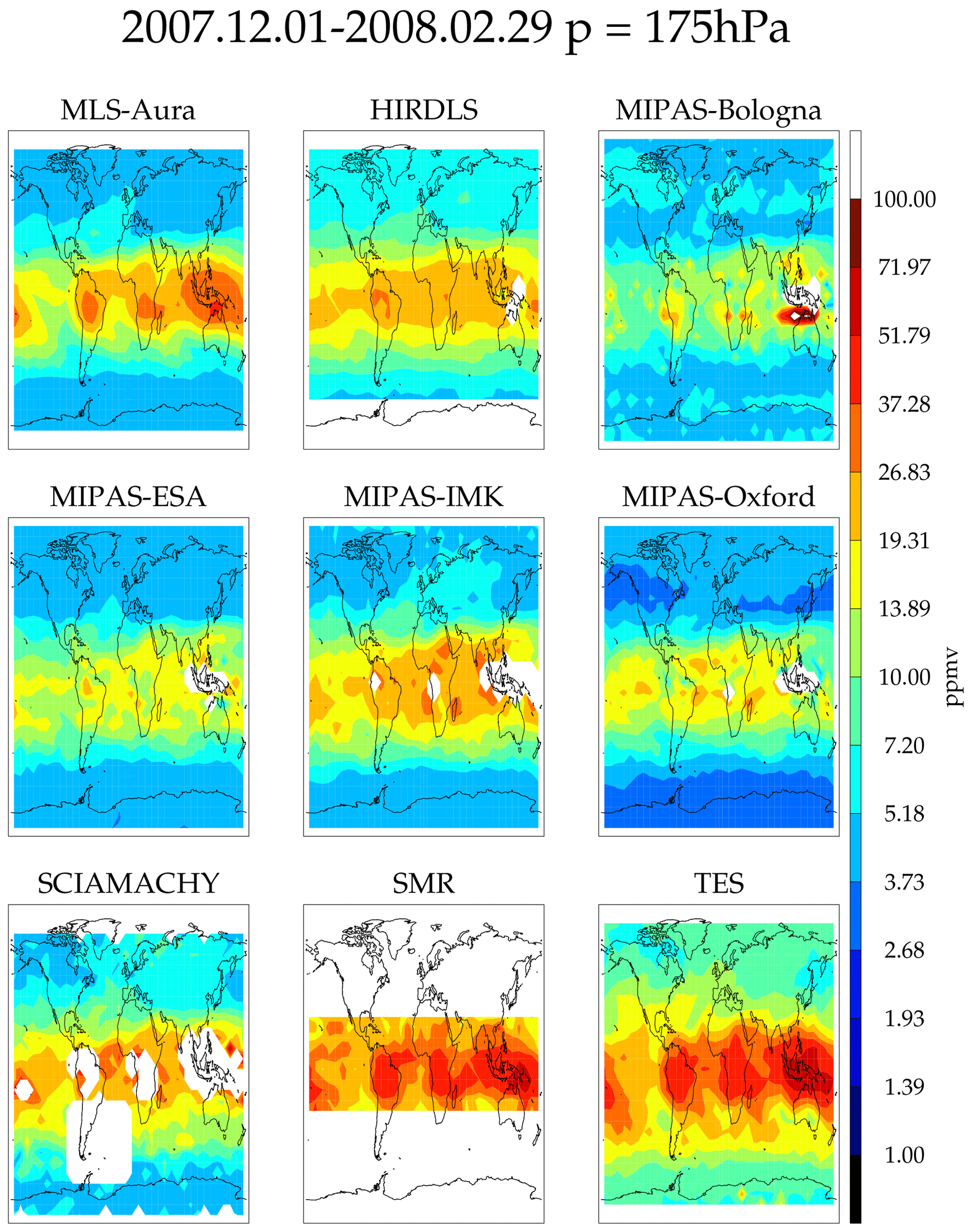
Figure 22 Gridded maps at 175 hPa generated from nine instruments. The time period is December 2007–February 2008.

Figure 23 shows a scatter plot of the mapped grid values with MLS-Aura on the x axis and various instruments on the y axis. The correlation is generally good between the instrument pairs. The MIPAS suite and HIRDLS are drier for moist values relative to MLS for reasons previously described. SCIAMACHY has no measurements in regions associated with active convection, probably because the UV backscatter is affected by even thinner clouds than the IR. TES and SMR are more moist than MLS-Aura for all values of humidity. Scatter plots for other heights are shown in the Supplement.

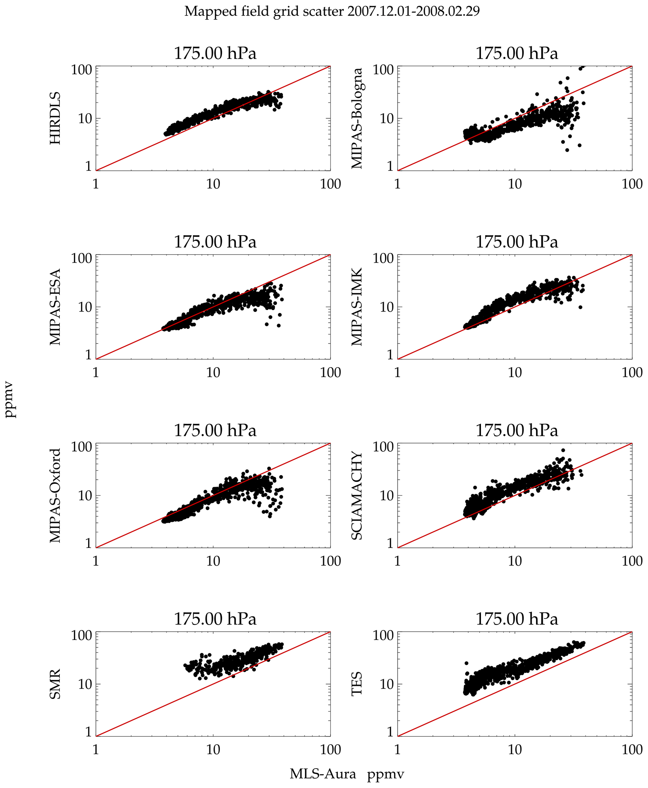
Figure 23 Scatter plot for 175 hPa and December 2007–February 2008 (MLS-Aura versus y instrument) of the map grid values in Fig. 22.

Another submillimeter radiometer, SMILES, has dense enough data coverage to produce climatological maps. SMILES operated for 6 months on the International Space Station (ISS). The instrument was not specifically designed to measure H₂O, but its radiances are affected by it, providing an opportunity for its measurement. Three independent humidity retrievals are available for SMILES using three different approaches. The NICT product retrieves H₂O from the line wing shape in its A and B radiometers. The JPL product fits the radiance growth curve in the window regions of each of its available radiometer bands (A, B, or C) relying on knowledge of the H₂O continuum function. The Chalmers product retrieves from the opaque downward-looking radiance, similar to its upper tropospheric humidity product on SMR. Table 1 gives the altitude ranges of these retrievals. The Supplement has maps showing these comparisons and scatter plots. Using MLS-Aura as a comparison standard, all these retrievals show significant biases; however, qualitatively, they do show the same patterns but over limited altitude ranges. A quick summary shows that the Chalmers retrieval produces good qualitative results from 280–200 hPa, the JPL retrieval does so from 200–125 hPa, and the NICT retrieval from 175–125 hPa. The NICT A band retrieval is much drier than the B band retrieval. The JPL retrievals suffer from high value artifacts at ∼45^∘ S that are not detected in quality screening. As mentioned previously, all these retrievals show significant (>factor of 2), usually moist, biases relative to MLS-Aura.

Climatologies for all of 2005 for several occultation instruments are compared to MLS-Aura. The sampling of the occultation instruments is much more sparse than it is for a passive thermal emission instrument. Moreover, many of these occultation instruments are set up in orbits to emphasize coverage in high latitudes in the interest of studying polar ozone chemistry. Therefore, despite the long gathering period and more coarse grids, such maps have lots of data gaps and inadequate data coverage. Maps and scatter plots for 200 and 150 hPa are in the Supplement. For the occultation instruments, the gridded map comparisons are in agreement with the other comparison methods.

6 Results

Figure 24 shows a quick-view summary of the comparisons done here. The figure is divided into two broad altitude regions: 300–200 hPa and 199–140 hPa. The figure shows results based on the three comparison methodologies: versus BFH sondes, inter-satellite coincidences, and mapped grid comparisons. The advantages and disadvantages of these comparison methodologies have been discussed. Moreover, not all three types of comparisons can be done for every data set, but by showing three methods, one can bridge one type of comparison (e.g., sonde) over to another (e.g., satellite coincidences). The “zero” difference reference is relative to the BFH sonde. The BFH sonde is an in situ hygrometer with a long historical operational record with an established track record and is currently accepted as an accurate (±10 %) hygrometer (Hurst et al., 2011) for measuring humidity down to sub ppmv concentrations. Due to the tight coincidence criterion (2.5^∘ longitude and latitude, 3 h time), a small number of instruments have enough coincidences (minimum of seven) to be assessed with spatial and temporal coincidences with BFH sondes. The width of the horizontal bar is a 1σ spread of the values among the six sonde sites used in this study. Coincidences are available for a subset of the BFH sites for some instruments. Thus, those instruments will have less geographical sampling in their assessment. The MIPAS retrieval suite, for example, has no coincidences with tropically located sondes. A summary of sondes and instruments with suitable coincidences is summarized in Fig. 6.

For those instruments for which there are direct sonde comparisons available, a mean bias can be established. For example, for MLS-Aura, it is −25 % for p>200 hPa and −31 % for p<200 hPa. When another instrument is compared to MLS-Aura in a satellite coincident or a gridded map comparison, the MLS–sonde bias is added to those comparison results in order to “correct” for the likely MLS dry bias relative to the BFHs.

The direct satellite-to-satellite coincidence comparisons use MLS-Aura, MIPAS-ESA, and MIPAS-IMK as the x-axis “reference instrument”. Exceptions are MAESTRO, which uses ACE-FTS and MLS-Aura for the reference instruments, and MLS-UARS, which uses SAGE-II. Since there is no direct coincidence sonde bias estimate for SAGE-II, there is no adjustment applied to that instrument's comparison results. The comparison statistics for the inter-satellite comparisons, in addition to being screened by the tropopause height, were binned by concentration amounts. The following bins are used: 0–10 ppmv, 10–50 ppmv, 50–100 ppmv, and >100 ppmv. Statistics are computed for each of these binned values and across the satellite reference suite (typically, MLS-Aura, MIPAS-ESA, and MIPAS-IMK). In many cases, results from all bins are not included as doing so would greatly skew the results when it is clear that the measurement of one of the instruments is poor. For example, the x-instrument's retrieved values establish the bin values, e.g., H₂O >100 ppmv. Such values are sparse and often outliers within that instruments retrieval and are probably overestimations of the true concentrations. The y-instrument values that are coincident will be considerably less as they are better quality retrievals in those instances. These are easily identified in plots like Figs. 17–19, where the correlation curve tends to zero slope. The same is also true for the low value bin <10 ppmv for instruments (MLS-UARS, p>200 hPa, SMILES-JPL, SMILES-Chalmers, SMR, and TES) that are not capable of measuring such low values. The parenthetical instruments are either nadir-like sounders requiring a thermal gradient or retrieve directly from the H₂O continuum. Dry stratospheric values are often near where the thermal lapse rate is small or its signal is dominated by other atmospheric continuum contributors like N₂ and O₂, both being sensitive to spectroscopic systematic errors.

Gridded map comparisons are handled similarly to the coincident satellite comparisons. MLS-Aura is used for the reference instrument in all cases except for assessing MLS-Aura itself. In that case AIRS is the reference instrument. Examples of gridded maps and their grid value scatter plots are shown in Figs. 20–23. Like the coincident satellite comparisons, the scatter plot statistics are derived from concentration bins set by the reference instrument. These are H₂O <10 ppmv, 10–50 ppmv, 50–100 ppmv and >100 ppmv. These comparisons are performed for 3-month climatologies for DJF 2007/8–SON 2008, except for SMILES which was done from DJFM 2009/10 because SMILES operated for a 6-month period in 2009–2010. As for the satellite coincidences, some bins were not included in the statistical assessment. Comparisons involving AIRS, SMILES-JPL, SMILES-Chalmers, and TES disregard results from the H₂O <10 ppmv bin. The infrared and UV–vis limb instruments are significantly cloud contaminated in the tropics; therefore, their sampling is greatly reduced there relative to the reference instrument MLS-Aura. Measurements from MLS-Aura, TES, AIRS, and SMR show that the cloud-impacted grids are the most moist. Therefore, comparison statistics in H₂O bins >100 ppmv at 250 hPa and H₂O bins >50 ppmv at 200–150 hPa are disregarded for the MIPAS suite and SCIAMACHY. After the comparison statistics are computed, they are shifted by the MLS-Aura dry bias relative to BFH as shown in Fig. 24. The spread of values represent a 1σ spread of the computed statistics for the pressure levels, H₂O bins, and seasons evaluated.

Figure 24 attempts to show possible satellite and Vaisala RS92 biases relative to BFH sondes with the assumption that the BFH represents the best accuracy standard for measuring humidity in the upper troposphere and lower stratosphere. The BFH hygrometer itself is considered to be accurate to 10 %. Figure 24 is the upper tropospheric equivalent to Fig. 1 in the first assessment report (Kley et al., 2000), summarizing the stratospheric humidity sensors in the pre-2000 era. The spread in the variability bar shown arises due to many factors such as location and concentration dependencies, sampling differences, possible averaging kernel smoothing effect dependencies on profile shape, and many possible systematic error contributions such as errors in atmospheric temperature and interfering species whose errors may not be uniform under all conditions that these comparisons are made in. Although an attempt has been made to reference these biases relative to the BFH, there are some inconsistencies. The mapped comparisons between MLS-Aura and AIRS typically show agreement within ±20 % for H₂O bins, pressures, and seasons considered. However, when the MLS-Aura dry bias relative to sonde is added it suggests that a climatological map produced by AIRS should have an overall dry bias of 20 %. The same gridded map comparison for MLS-Aura which is based on the same comparison with AIRS except that AIRS is the reference measurement shows only a slight (<10 %) dry bias. This is because the AIRS-to-BFH adjustment is −2 % and −6 % for the 300–200 hPa and 200–150 hPa levels, respectively, in Fig. 24. The cause of the differences relative to the BFH reference arises from MLS showing a strong bias dependence based on the height of the tropopause. In short, for pressure levels considered here, the MLS bias runs between near 0 % to 60 % when the tropopause is 2–3 km above the compared pressure level. The adjustment is roughly an average of these conditions. AIRS does not show this behavior; therefore, its bias adjustment is not tropopause height dependent and is therefore more robustly applicable. What is not included in Fig. 24 for the satellite coincident comparisons is an additional scatter resulting from the variability of paired differences and for the gridded maps, i.e., paired grid box value difference variability. These are typically ∼30 % for these comparisons; therefore, an additional ∼30 % variability would be added to that shown in Fig. 24 if one is to compare a single matched pair comparison.

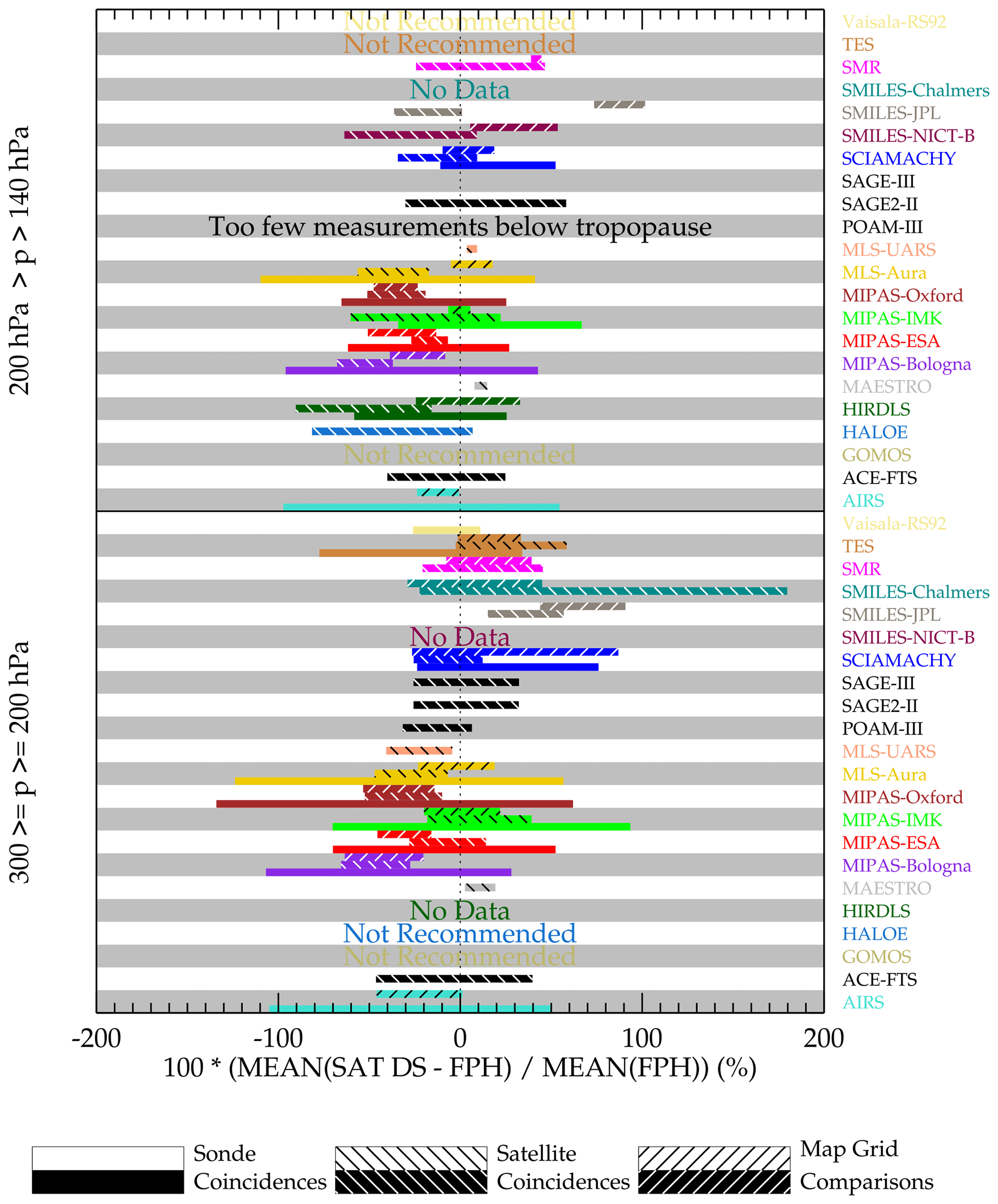
Figure 24 A summary plot of biases among the satellite and Vaisala RS92 sensor for the upper troposphere relative to BFH measurements (zero value on the x axis). The sonde coincidences have no hatching and are shown in the bottom third of the y axis band dedicated to the data set. The satellite coincidences and mapped grid comparisons have either black or white diagonal hatching, depending on the darkness of the data sets color and are shown in the middle and top third of the y axis dedicated to the data set.

UTH is a highly variable field in space and time. In the atmosphere, UTH can vary by a couple of orders of magnitude. Figure 24 shows that for most of the instruments, their comparisons among themselves and with BFH sondes are indicating mean agreement within ∼30 % but with large spreads, suggesting something like a factor of 2 agreement. Relative to stratospheric comparisons where H₂O is well mixed and it is possible to quantify biases to within a few percent, for the upper troposphere such a precise assessment is not realized. The problem is that the measurements sample atmospheric volumes differently where concentration gradients are large. The measurement systems have nonlinear responses to changes in water vapor amounts. The retrievals also require temperature in their inversion that also may have large vertical gradients. In short, it is probable that a comparison between two satellites or with balloon sondes (discussed earlier) will show different degrees of agreement for a large ensemble of coincident data, making it not possible to establish a single bias number by height and latitude.

7 Conclusions

To summarize, some features specific to certain instruments will be discussed. It is clear from the gridded map comparisons that high clouds in the tropical upper troposphere have a significant impact on infrared–ultraviolet limb viewers (see Table 1). While the limb geometry allows low concentrations of H₂O to be measured and does not require a negative thermal gradient, the long horizontal path length makes cloud encounters much more likely. The MIPAS retrieval suite and SCIAMACHY demonstrated good agreement with mid- and high-latitude sondes; however, their clear-sky sampling limitation causes a severe undersampling of the tropics, leading to a dry bias. This limitation was so severe that, for Fig. 24, moist value bins were not included in the assessment summary. Of course this limitation needs to be kept in mind for science investigations. The microwave limb viewers Aura, MLS-UARS, SMR, and SMILES are more immune to clouds due to the longer measurement wavelength being less subject to cloud emission and scattering. Nadir sounding geometries work better than limb geometries in cloudy scenes as the imaged scene is small compared to the horizontal distance covered by limb viewer and can look at scenes in close proximity to clouds without being contaminated by them. Also, AIRS by using highly spatially resolved pixels can use a cloud-clearing scheme to derive a cloud-free signal. Therefore, AIRS and TES although being infrared instruments can better observe in cloudy regions and avoid the severe sampling bias. As mentioned before, these instruments have a relatively short path length in the atmosphere and require a negative temperature gradient to measure humidity. Therefore, they are unable to make measurements ∼3 km below the tropopause and above or where H₂O concentrations are <10–20 ppmv.

Among the limb viewers, MLS-Aura has the highest daily sampling, is one of the longest running operations (still in operation), and is the least affected by clouds. Therefore, it was probably one of the better instruments to use as a reference for comparing the others, which was often done in this study. Having said that, the one significant feature is that MLS-Aura shows a significant dry bias (50 %) in any level that is ∼2.5 km below the tropopause. This bias reduces to <20 % above and below this critical level. The bias behavior is not caused by retrieval smoothing that can be corrected by including the averaging kernels. The cause is most likely due to a pointing error in the retrieval system. The pointing error is from a combination of two sources: one being a field-of-view alignment measurement and another from a sideband measurement. The needed adjustment for the field-of-view alignment is within its prelaunch uncertainty, but the sideband adjustment is ∼15 times larger than its prelaunch uncertainty, which confounded its discovery. Version 5 currently in production corrects for these deficiencies and will be shown in a future publication.

The occultation sounders can provide accurate profile measurements, with ACE-FTS being the best amongst them in terms of sampling a wide range of concentration values, a long operational period (still in operation), and producing accurate measurements. However, the high temporal and spatial variability of H₂O in the upper troposphere, along with the sparse sampling from occultation instruments, limits the usefulness of these measurements mostly to validation studies.

Instruments such as SMILES and HIRDLS had short operational lifetimes of 6 months and 3 years, respectively. The science that can be done with these measurements would be limited to features unique to those instruments. For example, HIRDLS has the best vertical resolution (1 km) among the satellite suite (typically 3 km). SMILES was mounted on the ISS; thus, its measurements sample the full diurnal cycle. This was exploited in a cloud study (Jiang et al., 2015). The water vapor products from SMILES are research products for which the instrument was not specifically designed to measure. Although qualitatively the mapped fields are mostly reasonable, biases are large and artifacts are present (see the Supplement for more details).

The last observation derived from this study refers to the goodness of the Vaisala RS92 radiosonde hygrometer in the uppermost troposphere. It is well known that the response time of the HUMICAP sensor in the Vaisala RS92 slows as the air becomes more desiccated (Miloshevich et al., 2009). This leads to erroneous measurements. Time-lag correction algorithms have been applied to some of these sondes, and only corrected sondes have been used here. This is in contrast to those used by the radiosonde network that uses an algorithm provided by Vaisala that does not have the time-lag correction. The motivation for including the Vaisala RS92 profiles was to greatly expand the number of Vaisala RS92 profiles available for more satellite data sets to be compared. Unfortunately, in the uppermost troposphere, the Vaisala RS92 radiosondes show inconsistent results and are therefore best not used for pressures less than 200 hPa. The agreement is much better for pressures between 300–200 hPa, but the data show a dry bias of 10 %. The expanded Vaisala RS92 data set does allow an assessment to be made for ACE-FTS, SMILES, and SMR. After correcting for the 10 % dry bias and only considering pressure levels >200 hPa, the mean agreement for ACE-FTS is 8 %, for SMILES-JPL is −10 %, and for SMR is 110 %. The variability of the differences between the Vaisala RS92 radiosonde and the satellite instruments is quite large (∼100 %).

In conclusion, with exceptions noted in the text, most of the satellite instruments do a realistic job of tracking upper tropospheric humidity changes. Precise quantitative assessment is much more difficult, because the nature of these measurements coupled with the sharp vertical and horizontal gradients in UTH leads to large variability of the coincident pair differences between the data sets. Even among the MIPAS suite of retrieval products, where the four retrieval products are using the same radiance signal, sampling exactly the same volume with perfect spatial and temporal coincidence shows surprisingly large biases and variability, underscoring significant sensitivities to the inverse models, profile smoothing constraints, a priori profile assumptions, and forward models. Science investigations using these data need to take these features into consideration and be aware of the sampling and measurement durations of these data sets (Table 1). Having said this, and ignoring some notable anomalies (e.g., MLS-Aura large dry bias in a 2–3 km layer below the tropopause) quantitatively, for most of the instruments, agreement within 20–30 % amongst each other with an additional variability of 30 % is being achieved. The list of instruments that consistently produce acceptable results is the following: ACE-FTS, AIRS, HIRDLS, MAESTRO, MIPAS-Bologna, MIPAS-ESA, MIPAS-IMK, MIPAS-Oxford, MLS-Aura, MLS-UARS, POAM-III, SAGE-II, SAGE-III, SCIAMACHY, SMR, and TES (p>200 hPa only). The SMILES suite is borderline in that it produces realistic results but is also subject to erroneous artifacts and can have very large biases and variability. HALOE is only good when the true atmospheric H₂O composition is <10 ppmv, which restricts it to the very uppermost troposphere and therefore is not generally useful for tropospheric humidity. The GOMOS upper tropospheric humidity product is not recommended.