the Creative Commons Attribution 4.0 License.
the Creative Commons Attribution 4.0 License.
 | 02 Nov 2022
Calibrating networks of low-cost air quality sensors
Priyanka deSouza
Ralph Kahn
Tehya Stockman
William Obermann
Ben Crawford
An Wang
James Crooks
Jing Li
Patrick Kinney
Ambient fine particulate matter (PM2.5) pollution is a major health risk. Networks of low-cost sensors (LCS) are increasingly being used to understand local-scale air pollution variation. However, measurements from LCS have uncertainties that can act as a potential barrier to effective decision making. LCS data thus need adequate calibration to obtain good quality PM2.5 estimates. In order to develop calibration factors, one or more LCS are typically co-located with reference monitors for short or long periods of time. A calibration model is then developed that characterizes the relationships between the raw output of the LCS and measurements from the reference monitors. This calibration model is then typically transferred from the co-located sensors to other sensors in the network. Calibration models tend to be evaluated based on their performance only at co-location sites. It is often implicitly assumed that the conditions at the relatively sparse co-location sites are representative of the LCS network overall and that the calibration model developed is not overfitted to the co-location sites. Little work has explicitly evaluated how transferable calibration models developed at co-location sites are to the rest of an LCS network, even after appropriate cross-validation. Further, few studies have evaluated the sensitivity of key LCS use cases, such as hotspot detection, to the calibration model applied. Finally, there has been a dearth of research on how the duration of co-location (short-term or long-term) can impact these results. This paper attempts to fill these gaps using data from a dense network of LCS monitors in Denver deployed through the city's “Love My Air” program. It offers a series of transferability metrics for calibration models that can be used in other LCS networks and some suggestions as to which calibration model would be most useful for achieving different end goals.
- Article
(10541 KB) - Full-text XML
-
Supplement
(2928 KB) - BibTeX
- EndNote


Poor air quality is currently the single largest environmental risk factor to human health in the world, with ambient air pollution being responsible for approximately 6.7 million premature deaths every year (Health Effects Institute, 2020). Having accurate air quality measurements is crucial for tracking long-term trends in air pollution levels, identifying hotspots, and developing effective pollution management plans. The dry-mass concentration of fine particulate matter (PM2.5), a criterion pollutant that poses more danger to human health than other widespread pollutants (Kim et al., 2015), can vary over distances as small as ∼ tens of meters in complex urban environments (Brantley et al., 2019; deSouza et al., 2020a). Therefore, dense monitoring networks are often needed to capture relevant spatial variations. Due to their costliness, Environmental Protection Agency (EPA) air quality reference monitoring networks are sparsely positioned across the US (Apte et al., 2017; Anderson and Peng, 2012).
Low-cost sensors (LCS) (< USD 2500, as defined by the US EPA Air Sensor Toolbox) (Williams et al., 2014) have the potential to capture concentrations of PM in previously unmonitored locations and to democratize air pollution information (Castell et al., 2017; Crawford et al., 2021; Kumar et al., 2015; Morawska et al., 2018; Snyder et al., 2013; deSouza and Kinney, 2021; deSouza, 2022). However, LCS measurements have several sources of greater uncertainty than reference monitors (Bi et al., 2020; Giordano et al., 2021; Liang, 2021).
Most low-cost PM sensors rely on optical measurement techniques. Optical instruments face inherent challenges that introduce potential differences in mass estimates compared to reference methods (Barkjohn et al., 2021; Crilley et al., 2018; Giordano et al., 2021; Malings et al., 2020):
-
Optical methods do not directly measure mass concentrations; rather, they estimate mass based on calibrations that convert light scattering data to particle number and mass. LCS come with factory-supplied calibrations but, in practice, must be re-calibrated in the field to ensure accuracy, due to variations in ambient particle characteristics and instrument drift.
-
High relative humidity (RH) can produce hygroscopic particle growth, leading to dry-mass overestimation, unless particle hydration can accurately be taken into account or the particles are desiccated by the instrument.
-
LCS are not able to detect particles with diameters below a specific size, which is determined by the wavelength of laser light within each device and is generally in the vicinity of 0.3 µm, whereas the peak in pollution particle number size distribution is typically smaller than 0.3 µm.
-
The physical and chemical parameters describing the aerosol (particle size distribution, shape, indices of refraction, hygroscopicity, volatility, etc.), which might vary significantly across different microenvironments with diverse sources, impact light scattering; this in turn affects the aerosol mass concentrations reported by these instruments.
The need for field calibration to correct LCS measurements is particularly important. This is typically done by co-locating a small number of LCS with one or a few reference monitors at a representative monitoring location or locations. The co-location could be carried out for a brief period before and/or after the actual study or may continue at a small number of sites for the duration of the study. In either case, the co-location provides data from which a calibration model that relates the raw output of the LCS as closely as possible to the desired quantity as measured by the reference monitor is developed. Thereafter, the calibration model is transferred to other LCS in the network based upon the presumption that ongoing sampling conditions are within the same range as those at the collocation site(s) during the calibration period.
Calibration models typically correct for (1) systematic error in LCS by adjusting for bias using reference monitor measurements, and (2) the dependence of LCS measurements on environmental conditions affecting the ambient particle properties, such as relative humidity (RH), temperature (T), and/or dew-point (D). Correcting for RH, T, and D is carried out through either (a) a physics-based approach that accounts for aerosol hygroscopic growth given particle composition using κ-Köhler's theory, or (b) empirical models, such as regression and machine learning techniques. In this paper, we focus on the latter, as it is currently the most widely used (Barkjohn et al., 2021). Previous work has also shown that the two approaches yield comparable improvements in the case of PM2.5 LCS (Malings et al., 2020).
Prior studies have used multivariate regressions, piecewise linear regressions, or higher order polynomial models to account for RH, T, and D in these calibration models (Holstius et al., 2014; Magi et al., 2020; Zusman et al., 2020). More recently, machine learning techniques such as random forests, neural networks, and gradient-boosted decision trees have been used (Considine et al., 2021; Liang, 2021; Zimmerman et al., 2018). Researchers have also started including additional covariates in their models besides that which is directly measured by the LCS, such as time of day, seasonality, wind direction, and site type, which have been shown to yield significantly improved results (Considine et al., 2021).
Past research has shown that there are several important decisions in addition to the choice of calibration model that need to be made during calibration and that can impact the results (Bean, 2021; Giordano et al., 2021; Hagler et al., 2018). These include (a) the kind of reference air quality monitor used, (b) the time interval (e.g., hour or day) over which to average measurements used when developing the calibration model, (c) how cross-validation (e.g., leaving one site out or 10-fold cross-validation) is carried out, and (d) how long the co-location experiment takes place.
Calibration models are typically evaluated based on how well the corrected data agree with measurements from reference monitors at the corresponding co-location site. A commonly used metric is the Pearson correlation coefficient, R, which quantifies the strength of the association. However, it is a misleading indicator of sensor performance when measurements are observed close to the limit of detection of the instrument. Therefore, root mean square error (RMSE) is often included in practice. Unfortunately, neither of these metrics captures how well the calibration method developed at the co-located sites transfers to the rest of the network in both time and space.
If the conditions at the co-location sites (meteorological conditions, pollution source mix) for the period of co-location are the same as for the rest of the network during the total operational period, the calibration model developed at the co-location sites can be assumed to be transferable to the rest of the network. In order to ensure that the sampling conditions at the co-location site are representative of sampling conditions across the network, most researchers tend to deploy monitors in the same general sampling area as the network (Zusman et al., 2020). However, it is difficult to definitively test if the co-location site during the period of co-location is representative of conditions at all monitors in the network; ambient PM concentrations can vary on scales as small as a few meters. Furthermore, LCS are often deployed specifically in areas where the air pollution conditions are poorly understood, meaning that representativeness cannot be assessed in advance.
In order to evaluate whether calibration models are transferable in time, we test if models generated using typical short-term co-locations at specific co-location sites perform well during other time periods at all co-location sites. Where multiple co-location sites exist, one way to evaluate how transferable calibration models are in space is to leave out one or more co-location sites and to test if the calibration model is transferable to the left-out sites. This method was used in recent work evaluating the feasibility of developing a US-wide calibration model for the PurpleAir low-cost sensor network (Barkjohn et al., 2021; Nilson et al., 2022).
Although these approaches are useful, co-location sites are sparse relative to other sites in the network. Even in the PurpleAir network (which is one of the densest low-cost networks in the world), there were only 39 co-location sites in 16 US states, a small fraction of the several thousand PurpleAir sites overall (Barkjohn et al., 2021). It is thus important to develop metrics to test how sensitive the spatial and temporal trends of pollution derived from the entire network are to the calibration model applied. Finally, a key use case of LCS networks is to identify hotspots. It is important to also evaluate how sensitive the hotspot identified in an LCS network is to the calibration model applied.
Examining the reliability of calibration models is timely, because more researchers are opting to use machine learning models. Although in most cases, such models have yielded better results than traditional linear regressions, it is important to examine if these models are overfitted to conditions at the co-location sites, even after appropriate cross-validation, and how transferable they are to the rest of the network. Indeed, because of concerns of overfitting, some researchers have explicitly eschewed employing machine learning calibration models altogether (Nilson et al., 2022). It is important to test under what circumstances such concerns might be warranted.
This paper uses a dense low-cost PM2.5 monitoring network deployed in Denver, the “Love My Air” network deployed primarily outside the city's public schools, to evaluate the transferability of different calibration models in space and time across the network. To do so, new metrics are proposed to quantify the Love My Air network's spatial and temporal trend uncertainty due to the calibration model applied. Finally, for key LCS network use cases, such as hotspot detection, tracking high pollution events, and evaluating pollution trends at a high temporal resolution, the sensitivity of the results to the choice of calibration model is evaluated. The methodologies and metrics proposed in this paper can be applied to other low-cost sensor networks, with the understanding that the actual results will vary with study region.
2.1 Data sources
Between 1 January and 30 September 2021, Denver's Love My Air sensor network collected minute-level data from 24 low-cost sensors deployed across the city outside of public schools and at 5 federal equivalent method (FEM) reference monitor locations (Fig. 1). The Love My Air sensors are Canary-S models, equipped with a Plantower 5003, made by Lunar Outpost Inc. The Canary-S sensors detect PM2.5, T, and RH and upload minute-resolution measurements to an online platform via cellular data network.

Figure 1Locations of all 24 Love My Air sensors. Sensors displayed with an orange triangle indicate that they were co-located with a reference monitor. The labels of the co-located sensors include the name of the reference monitor with which they were co-located after a hyphen.
We found that RH and T reported by the Love My Air sensors were well correlated with that reported by the reference monitoring stations. We used the Love My Air LCS T and RH measurements in our calibration models, as they most closely represent the conditions experienced by the sensors.
2.1.1 Data cleaning protocol for measurements from the Love My Air network
A summary of the data cleaning and data preparation steps carried out on the Love My Air data from the entire network are listed below:
-
We removed data for time steps where key variables (PM2.5, T, and RH measurements) were missing.
-
We removed unrealistic RH and T values (RH <0 and ∘C).
-
We removed PM2.5 values above 1500 µg m−3 (outside the operational range of the Plantower sensors used) from the Canary-S sensors (Considine et al., 2021).
-
We were left with 8 809 340 min-level measurements and then calculated hourly average PM2.5, T, and RH measurements for each sensor; we had a total of 147 101 hourly averaged measurements.
-
From inspection, one of the monitors, CS13, worked intermittently in January and February before resuming continuous measurement in March (Fig. S1 in the Supplement). When CS13 worked intermittently, large spikes in the measurements were observed, likely due to power surges. We thus retained measurements taken after 1 March 2021 for this monitor. The total number of hourly measurements was thus reduced to 146 583.
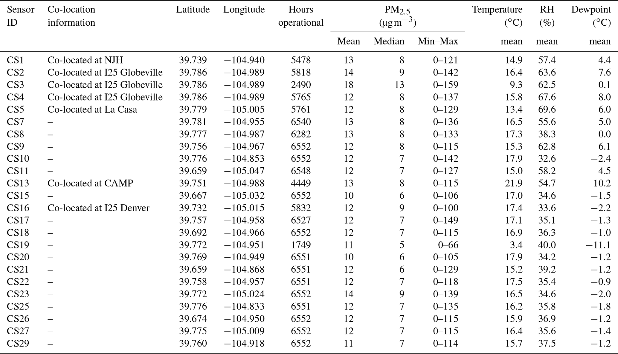
Love My Air sensors (indicated by Sensor ID) were co-located with FEM reference monitors, from which we obtained high-quality hourly PM2.5 measurements, at the following locations (Table 1):
-
La Casa (Sensor ID: CS5)
-
CAMP (Sensor ID: CS13)
-
I25 Globeville (Sensor ID: CS2, CS3, CS4)
-
I25 Denver (Sensor ID: CS16)
-
NJH (Sensor ID: CS1) for the entire period of the experiment.
Table 1Site location of each Love My Air sensor, as well as summary statistics of hourly measurements from each sensor.
2.1.2 Data preparation steps for preparing a training dataset used to develop the various calibration models
A summary of the data preparation steps for preparing a training dataset used to develop the various calibration models is described below:
-
We joined hourly averages from each of the seven co-located Love My Air monitors with the corresponding FEM monitor. We had a total of 35 593 co-located hourly measurements for which we had data for both the Love My Air sensor and the corresponding reference monitor. Figure S2 displays time-series plots of PM2.5 from all co-located Love My Air sensors. Figure S3 displays time-series plots of PM2.5 from the corresponding reference monitors.
-
The three Love My Air sensors co-located at the I25 Globeville sites (CS2, CS3, CS4) agreed well with each other (Pearson correlation coefficient =0.98) (Figs. S4 and S5). To ensure that our co-located dataset was well balanced across sites, we only retained measurements from CS2 at the I25 Globeville site. We were left with a total of 27 338 co-located hourly measurements that we used to develop a calibration model. Figure S6 displays the time-series plots of PM2.5 from all other Love My Air sensors in the network.
Reference monitors at La Casa, CAMP, I25 Globeville, and I25 Denver also reported minute-level PM2.5 concentrations between 23 April, 11:16, and 30 September, 22:49 local time. We also joined minute-level Love My Air PM2.5 concentrations with minute-level reference data at these sites. We had a total of 1 062 141 co-located minute-level measurements during this time period. As with the hourly averaged data, we only retained data from one of the Love My Air sensors at the I25 Globeville site and were thus left with 815 608 min-level measurements from one LCS at each of the four co-location sites.
Table S1 in the Supplement has information on the minute-level co-located measurements. The data at the minute-level displays more variation and peaks in PM2.5 concentrations than the hourly averaged measurements (Fig. S7), likely due to the impact of passing sources. It is also important to mention that minute-level reference data may have some additional uncertainties introduced due to the finer time resolution. We will use the minute-level data in the Supplement analyses only. Thus, unless explicitly referenced, we will be reporting results from hourly averaged measurements.
2.1.3 Deriving additional covariates
We derived dew point (D) from T and RH reported by the Love My Air sensors using the weathermetrics package in the programming language R (Anderson and Peng, 2012), as D has been shown to be a good proxy of particle hygroscopic growth in previous research (Barkjohn et al., 2021; Clements et al., 2017; Malings et al., 2020). Some previous work has also used a nonlinear correction for RH in the form of , which we also calculated for this study (Barkjohn et al., 2021).
We extracted hour, weekend, and month variables from the Canary-S sensors and converted hour and month into cyclic values to capture periodicities in the data by taking the cosine and sine of hour × and month × , which we designate as cos_time, sin_time, cos_month, and sin_month, respectively. Sinusoidal corrections for seasonality have been shown to improve the accuracy of PM2.5 measurements in machine learning models (Considine et al., 2021).
2.2 Defining the calibration models used
The goal of the calibration model is to predict, as accurately as possible, the “true” PM2.5 concentrations given the concentrations reported by the Love My Air sensors. At the co-located sites, the FEM PM2.5 measurements, which we take to be the “true” PM2.5 concentrations, are the dependent variable in the models.
We evaluated 21 increasingly complex models that included T, RH, and D as well as metrics that captured the time-varying patterns of PM2.5 to correct the Love My Air PM2.5 measurements (Tables 2 and 3).
Sixteen models were multivariate regression models that were used in a recent paper (Barkjohn et al., 2021) to calibrate another network of low-cost sensors: the PurpleAir, which relies on the same PM2.5 sensor (Plantower) as the Canary-S sensors in the current study. As T, RH, and D are not independent (Fig. S8), the 16 linear regression models include adding the meteorological conditions considered as interaction terms instead of additive terms. The remaining five calibration models relied on machine learning techniques.
Machine learning models can capture more complex nonlinear effects (for instance, unknown relationships between additional spatial and temporal variables). We opted to use the following machine learning techniques: random forest (RF), neural network (NN), gradient boosting (GB), SuperLearner (SL); these have been widely used in calibrating LCS. A detailed description of each technique can be found in Sect. S1 in the Supplement. All machine learning models were run using the caret package in R (Kuhn et al., 2020).
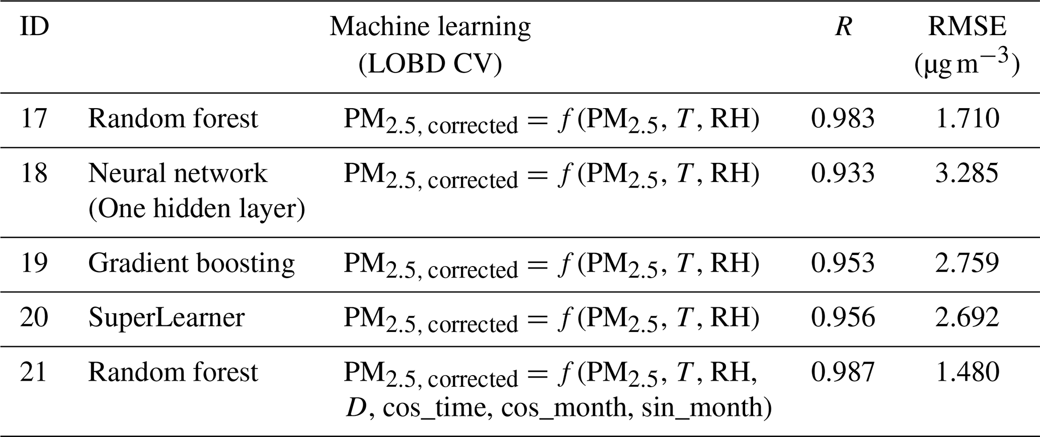
We used both leave-one-site-out (LOSO) (Table 2) and leave-out-by-date – where we left out a three-week period of data at a time at all sites (LOBD) (Table 3) – cross-validation (CV) methods to avoid overfitting in the machine learning models. For more details on the cross-validation methods used to avoid overfitting in the machine learning models, refer to Sect. S2.
Table 2Performance of the calibration models as captured using root mean square error (RMSE) and Pearson correlation (R). LOSO CV was used to prevent overfitting in the machine learning models. All corrected values were evaluated over the entire time period (1 January–30 September 2021).
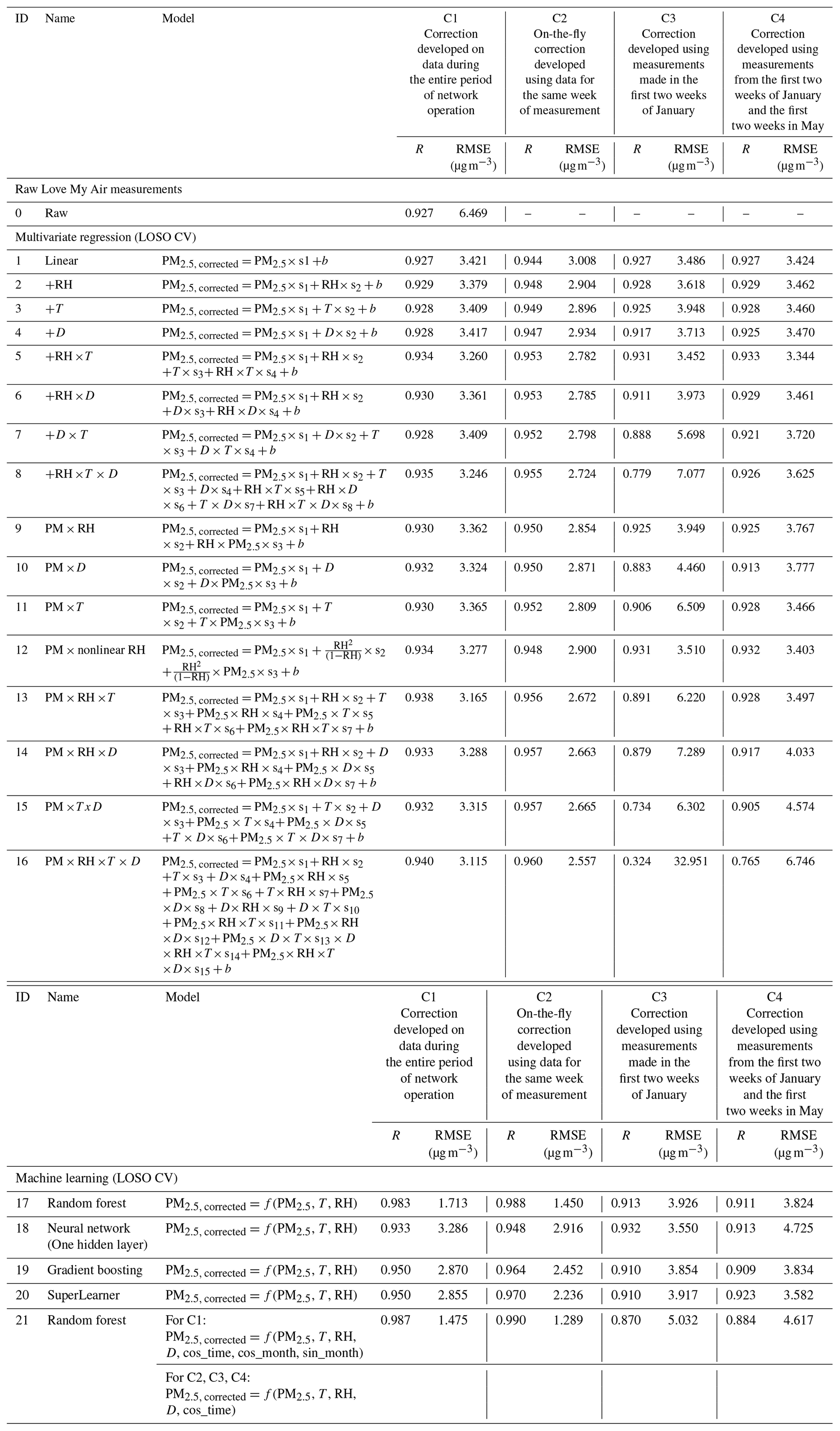
Table 3Performance of the calibration models using the C1 correction as captured using root mean square error (RMSE) and Pearson correlation (R). LOBD CV was used to prevent overfitting in the machine learning models.
Corrections generated using different co-location time periods (long-term, on-the-fly, short-term)
As described earlier, co-location studies in the LCS literature have been conducted over different time periods. Some studies co-locate one or more LCS for brief periods of time before or after an experiment, whereas others co-locate a few LCS for the entire duration of the experiment. These studies apply calibration models generated using the co-located data to measurements made by the entire network over the entire duration of the experiment. We attempt to replicate these study designs in our experiment to evaluate the transferability of calibration models across time by generating four different corrections:
- C1
Entire dataset correction. The 21 calibration models were developed using data at all co-location sites for the entire period of co-location.
- C2
On-the-fly correction. The 21 calibration models to correct a measurement during a given week were developed using data across all co-located sites for the same week of the measurement.
- C3
Two-week winter correction. The 21 calibration models were developed using co-located data collected for a brief period (two weeks) at the beginning of the study (1–4 January 2021). They were then applied to measurements from the network during the rest of the period of operation.
- C4
Two-week winter + two-week spring. The 21 calibration models were developed using co-located data collected for two two-week periods in different seasons (1–4 January 2021 and 1–14 May 2021). They were then applied to measurements from the network during the rest of the period of operation.
Although models developed using co-located data over the entire time period (C1) tend to be more accurate over the entire spatiotemporal dataset, it is inefficient to re-run large models frequently (incorporating new data). On-the-fly corrections (such as C2) can help characterize short-term variation in air pollution and sensor characteristics. The duration of calibration is a key question that remains unanswered (Liang, 2021). We opted to test corrections C3 and C4, as many low-cost sensor networks rely on developing calibration models based on relatively short co-location periods (deSouza et al., 2020b; West et al., 2020; Singh et al., 2021). Each of the 21 calibration models considered was tested under four potential correction schemes (C1, C2, C3, and C4).
For C1, the five machine learning models were trained using two CV approaches: LOSO and LOBD, separately. For C2, C3, and C4, only LOSO was conducted, as model application is already being performed on a different time period from the training (for more details, refer to Sect. S2). Overall, we tested 89 calibration models listed in Tables 2 and 3.
2.3 Evaluating the calibration models developed under the four different correction schemes
We first qualitatively evaluate transferability of the calibration models from the co-location sites to the rest of the network by comparing the distribution of T and RH at the co-location sites during time-periods used to construct the calibration models with that experienced over the entire course of network operation (Fig. 2).
We then evaluate how well different calibration models perform when using the traditional methods of model evaluation (Tables 2, 3, S2). We attempt to quantify the degree of transferability of the calibration models in time by asking how well calibration models developed during short-term co-locations (corrections: C3 and C4) perform when transferred to long-term network measurements. To answer this question, we evaluated calibration models using corrections C3 and C4 only for the time period over which the calibration models were developed, which was 1–4 January 2021 for C3, and 1–4 January 2021 and 1–14 May 2021 for C4 (Table S2). We compared the performance of C3 and C4 corrections during this time period with that obtained from applying these models over the entire time period of the network (Table 2).
We next ask how well calibration models developed at a small number of co-locations sites transfer in space to other sites using the methodology detailed in the next subsection.
2.3.1 Evaluating transferability of calibration models over space
To evaluate how transferable the calibration technique developed at the co-located sites was to the rest of the network, we left out each of the five co-located sites in turn and, using data from the remaining sites, ran the models proposed in Tables 2 and 3. We then applied the models generated to the left-out site. We report the distribution of RMSE from each calibration model considered at the left-out sites using box plots (Fig. 3). For correction C1, we also left out a three-week period of data at a time and generated the calibration models based on the data from the remaining time periods at each site. For the machine learning models (Models 17–21), we used CV = LOBD. We plotted the distribution of RMSE from each model considered for the left-out three-week period (Fig. 3).
We statistically compare the errors in predictions for each test dataset with errors in predictions from using all sites in our main analysis. Such an approach is useful for understanding how well the proposed correction can transfer to other areas in the Denver region. To compare statistical differences between errors, we used t tests if the distribution of errors were normally distributed (as determined by a Shapiro–Wilk test); if not, we used Wilcoxon signed rank tests, using a significance value of 0.05.
We have only five co-location sites in the network. Although evaluating the transferability among these sites is useful, as we know the true PM2.5 concentrations at these sites, we also evaluated the transferability of these models in the larger network by predicting PM2.5 concentrations using the models proposed in Tables 2 and 3 at each of the 24 sites in the Love My Air network. For each site, we display time series plots of corrected PM2.5 measurements in order to visually compare the ensemble of corrected values at each site (Fig. 4).
We next propose different metrics to quantify the uncertainty in spatial and temporal trends in PM2.5 reported by the LCS network as introduced by the choice of calibration model applied in the subsection below.
2.3.2 Evaluating sensitivity of the spatial and temporal trends of the low-cost sensor network to the method of calibration
We evaluate the spatial and temporal trends in the PM2.5 concentrations corrected using the 89 different calibration models, using similar methods to those described in Jin et al. (2019) and deSouza et al. (2022) by calculating the following:
-
The spatial root mean square difference (RMSD) (Fig. 5) between any two corrected exposures at the same site: , where Conchi and Concdi are 1 January–30 September 2021 averaged PM2.5 concentrations estimated from correction h and d for site i. N is the total number of sites.
-
The temporal RMSD (Fig. 6) between pairs of exposures: , where Concht and Concdt are hourly corrected PM2.5 concentrations averaged over all operational Love My Air sites, estimated from correction h and d for time t. M is the total number of hours of operation of the network.
We characterized the uncertainty in the “corrected” PM2.5 estimates at each site across the different models using two metrics: a normalized range (NR) (Fig. 7a) and uncertainty, calculated from the 95 % confidence interval (CI), assuming a t statistical distribution (Fig. 7b). NR for a given site represents the spread of PM2.5 across the different correction approaches.
-
.
Ckt is the PM2.5 concentration at hour t from the kth model from the ensemble of K (which, in this case, is 89) correction approaches. represents the ensemble mean across the K different products at hour t. M is the total number of hours in our sample for which we have PM2.5 data for the site under consideration.
For our sample (K=89), we assume that the variations in PM2.5 across multiple models follows the Student t distribution, with the mean being the ensemble average. The confidence interval (CI) for the ensemble mean at a given time t is , where represents the ensemble mean at time t; t* is the upper critical value for the t distribution with K-1 degrees of freedom. For K=89, t* for the 95 % double-tailed confidence interval is 1.99. SDt is the sample standard deviation at time t. .
-
We define an overall estimate of uncertainty as follows: , which can also be expressed as .
2.3.3 Evaluating the sensitivity of hotspot detection across the network of sensors to the calibration method
One of the key use cases of low-cost sensors is hotspot detection. We report the labels of sites that are the most polluted using calibrated measurements from the 89 different models using hourly data. We repeat this process for daily, weekly, and monthly averaged calibrated measurements. We ignore missing measurements from the network when calculating time-averaged values for the different time periods considered. We report the mean number of sensors that are ranked “most polluted” across the different correction functions for the different averaging periods (Fig. 8). We do this to identify if the choice of the calibration model impacts the hotspot identified by the network (i.e., depending on the calibration model, different sites show up as the most polluted).
2.3.4 Supplementary analysis: evaluating transferability of calibration models developed in different pollution regimes
We evaluated model performance for true and reference PM2.5 concentrations >30 µg m−3 and ≤30 µg m−3, as Nilson et al. (2022) have shown that calibration models can have different performances in different pollution regimes. We chose to use 30 µg m−3 as the threshold, as these concentrations account for the greatest differences in health and air pollution avoidance behavior impacts (Nilson et al., 2022). Lower concentrations (PM2.5≤30 µg m−3) represent most measurements observed in our network; better performance at these levels will ensure better day-to-day functionality of the correction. High PM2.5 (>30 µg m−3) concentrations in Denver typically occur during fires. Better performance of the calibration models in this regime will ensure that the LCS network can accurately capture pollution concentrations under smoky conditions. In order to compare errors observed in the two different concentration ranges, in addition to reporting R and RMSE of the calibration approaches, we also report the normalized RMSE (normalized by the mean of the true concentrations) (Tables S3 and S4).
2.3.5 Supplementary analysis: evaluating transferability of calibration models developed across different time aggregation intervals
One of the key advantages of LCS is that they report high frequency (timescales shorter than an hour) measurements of pollution. As reference monitoring stations provide hourly or daily average pollution values, most often, the calibration model is developed using hourly averaged data and is then applied to the unaggregated, high-frequency LCS measurements. We applied the calibration models described in Tables 2 and 3 developed using hourly averaged co-located measurements on minute-level measurements from the co-located LCS described in Table S1. We evaluated the performance of the corrected high-frequency measurements against the “true” measurements from the corresponding reference monitor using the metrics R and RMSE (Tables S5 and S6).
We first report how representative meteorological conditions at the co-located sites were of the overall network. Temperature at the co-located sites across the entire period of the experiment (from 1 January to 30 September 2021) were similar to those at the rest of Love My Air network (Fig. 2a). The sensor CS19 is the only one that recorded lower temperatures than those at any of the other sites, likely due to it being in the shade. Relative humidity at the co-located sites (three of the four co-located sites have a median RH close to 50 % or higher) is higher than at the other sites in the network (7 of the 12 other sites have a median RH <50 %) (Fig. 2b). The similarity in meteorological conditions at the co-located sites with those experienced by the rest of the network suggests that models developed using long-term data (C1) are likely to be transferable to the overall network.
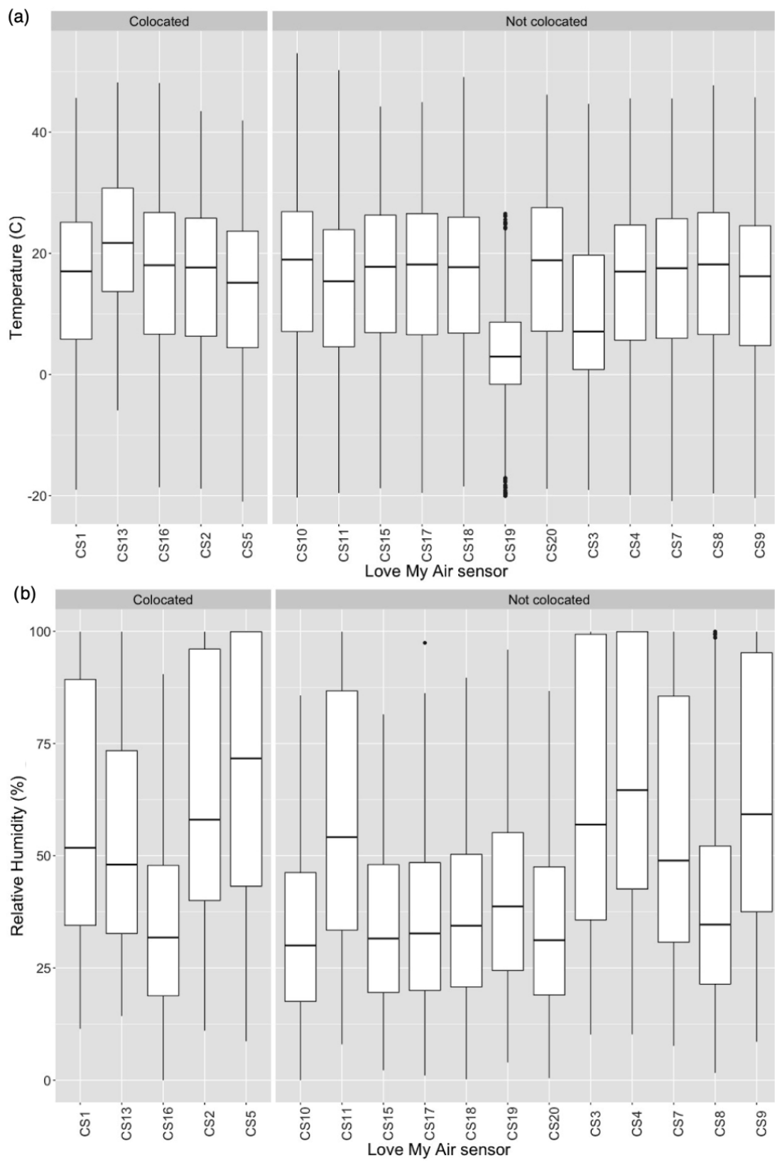
Figure 2(a) Distribution of temperature recorded by each Love My Air sensor, (b) Distribution of RH recorded by each Love My Air sensor. The distribution of temperature and RH recorded by co-located LCS is shown on the left. The distribution of temperature and RH recorded by all LCS not used to construct the calibration models are displayed on the right.
We also compared meteorological conditions during the development of corrections C3 (1–4 January 2021) and C4 (1–4 January 2021 and 1–14 May 2021) to those measured during the duration of network operation (C3: Figs. S10 and S11; C4: Figs. S12 and S13). Unsurprisingly, temperatures at the co-located sites during the development of C4 were more representative of the network than C3, although they were, on average, lower (median temperatures ∼ 10–17∘C) than the average temperatures experienced by the network (median temperatures ∼ 5–23∘C). RH values at co-located sites during C3 and C4 tend to be higher than conditions experienced by Love My Air sensors CS8, CS10, CS15, CS16, CS17, CS18, and CS20, likely due to the different microenvironments experienced at each site. The differences in meteorological conditions at the co-located sites for the time period of calibration model developed with those experienced by the rest of the network suggest that models developed using short-term data (C3, C4) are not likely to be transferable to the overall network.
When we evaluate the performance of applying each of the 89 calibration models on all co-located data, we find that, based on R and RMSE values, the on-the-fly C2 correction performed better overall than the C1, C3, and C4 corrections for most calibration model forms (Tables 2 and 3).
Within corrections C1 and C2, we found that an increase in complexity of the model form resulted in a decreased RMSE. Overall, Model 21 yielded the best performance (RMSE =1.281 µg m−3 when using the C2 correction, 1.475 µg m−3 when using the C1 correction with a LOSO CV, and 1.480 µg m−3 when using a LOBD correction). In comparison, the simplest model yielded an RMSE of 3.421 µg m−3 for the C1 correction and 3.008 µg m−3 when using the C2 correction. For correction C1, using a LOBD CV (Table 3) with the machine learning models resulted in better performance than using a LOSO CV (Table 2), except for Model 21, which is an RF model with additional time-of-day and month covariates, for which performance using the LOSO CV was marginally better (RMSE: 1.475 µg m−3 versus 1.480 µg m−3).
We also found that, for corrections of short-term calibrations (C3 and C4), more complex models yielded a better performance (for example the RMSE for Model 16: 2.813 µg m−3, RMSE for Model 2: 3.110 µg m−3, generated using the C3 correction) when evaluated alone during the period of co-location (Table S2). However, when models generated using the C3 and C4 corrections were transferred to the entire time period of co-location, we found that more complex multivariate regression models (Models 13–16) and the machine learning model (Model 21) that include cos_time performed significantly worse than the simpler models (Table 2). In some cases, these models performed worse than the uncorrected measurements. For example, applying Model 16 generated using C3 on the entire dataset resulted in an RMSE of 32.951 µg m−3 compared to 6.469 µg m−3 for the uncorrected measurements.
Including data from another season, spring, in addition to winter in the training sample (C4) resulted in significantly improved performance of calibration models over the entire dataset compared to C3 (winter), although it did not result in an improvement in performance for all models compared to the uncorrected measurements. For example, Model 16 generated using C4 yielded an RMSE of 6.746 µg m−3. Among the multivariate regression models, we found that models of the same form that corrected for RH instead of T or D did best. The best performance was observed for models that included the nonlinear correction for RH (Model 12) or included an RH ×T term (Model 5) (Table 2).
3.1 Evaluating transferability of the calibration algorithms in space
Large reductions in RMSE are observed when applying simple linear corrections (Models 1–4) developed using a subset of the co-located data to the left-out sites (Fig. 3a, c, d, e) or time periods (Fig. 3b) across C1, C2, C3, and C4. Increasing the complexity of the model does not result in marked changes in correction performance on different test sets for C1 and C2. Although the performance of the corrected datasets did improve on average for some of the complex models considered (Models 17, 20, 21, for example, vis-a-vis simple linear regressions when using the C1 correction) (Fig. 3a, b), this was not the case for all test datasets considered, as evidenced by the overlapping distributions of RMSE performances (e.g., Model 11 using the C2 correction resulted in a worse fit for one of the test datasets). For C3 and C4, the performance of corrections was worse across all datasets for the more complex multivariate model formulations (Fig. 3d, e), indicating that using uncorrected data is better than using these corrections and calibration models.
Wilcoxon tests and t tests (based on whether Shapiro–Wilk tests revealed that the distribution of RMSEs was normal) revealed significant improvements in the distribution of RMSEs for all corrected test sets vis-a-vis the uncorrected data. Across the different models, there was no significant difference in the distribution of RMSE values from applying C1 and C2 corrections to the test sets. For corrections C3 and C4, we found significant differences in the distribution of RMSEs obtained from running different models on the data, implying that the choice of model has a significant impact on transferability of the calibration models to other monitors.
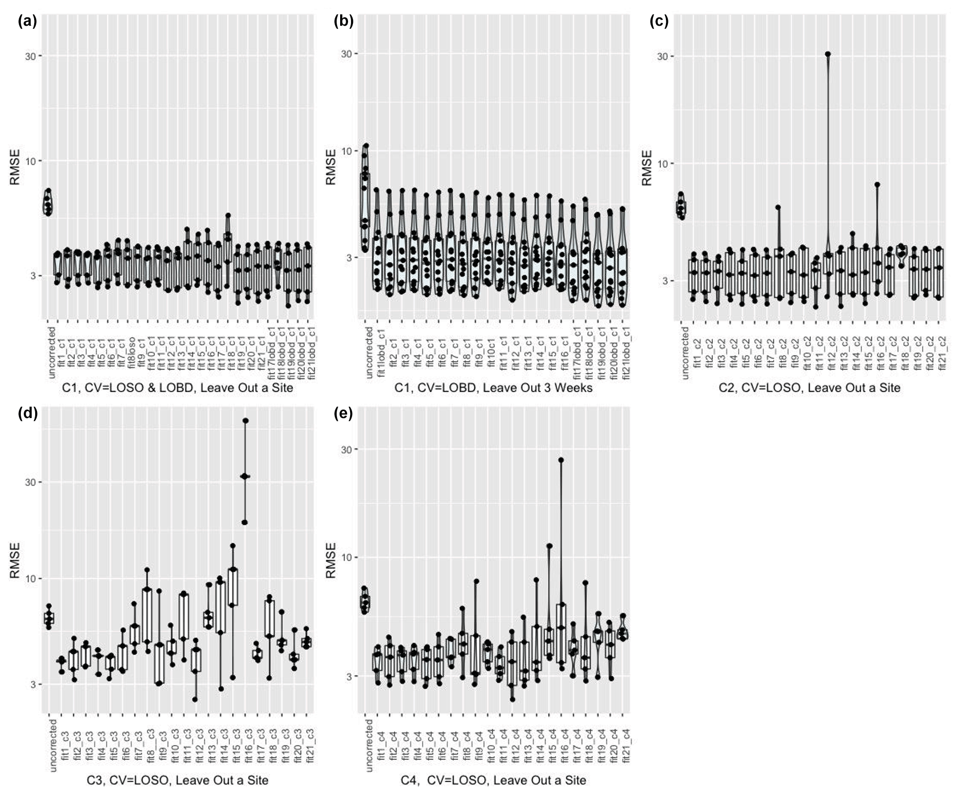
Figure 3Performance (RMSE) of corrected Love My Air PM2.5 data by generating corrections based on the 21 models (designated as fit) previously proposed using (a) correction C1 when leaving out a co-location site in turn and then running the generated correction on the test site (note that for machine learning models (Models 17–21), we performed CV using a LOSO CV as well as a LOBD CV approach.); (b) correction C1 when leaving out three-week periods of data at a time and generating corrections based on the data from the remaining time periods across each site, and evaluating the performance of the developed corrections on the held-out three weeks of data (note that for machine learning models (Models 17–21), we performed CV using a LOBD CV approach); (c) correction C2 when leaving out a co-location site in turn and then running the generated correction on the test site; (d) correction C3 when leaving out a co-location site in turn and then running the generated correction on the test site; (e) correction C4 when leaving out a co-location site in turn and then running the generated correction on the test site. Each point represents the RMSE for each test dataset permutation. The distribution of RMSEs is displayed using box plots and violin plots.
The time series of corrected PM2.5 values for Models 1, 2, 5, 16, and 21 (RF using additional variables) (using CV = LOSO for the machine learning Models 17 and 21) for corrections generated using C1, C2, C3, and C4 are displayed in Fig. 4 for Love My Air sensor CS1. These subsets of models were chosen, as they cover the range of model forms considered in this analysis.
From Fig. 4, we note that, although the different corrected values from C1 and C2 track each other well, there are small systematic differences between the different corrections. Peaks in corrected values using C2 tend to be higher than those using C1. Peaks in corrected values using machine learning methods using C1 are higher than those generated from multivariate regression models. Figure 4 also shows marked differences in the corrected values from C3 and C4. Specifically, Model 16 yields peaks in the data that corrections using the other models do not generate. This pattern was consistent when applying this suite of corrections to other Love My Air sensors.
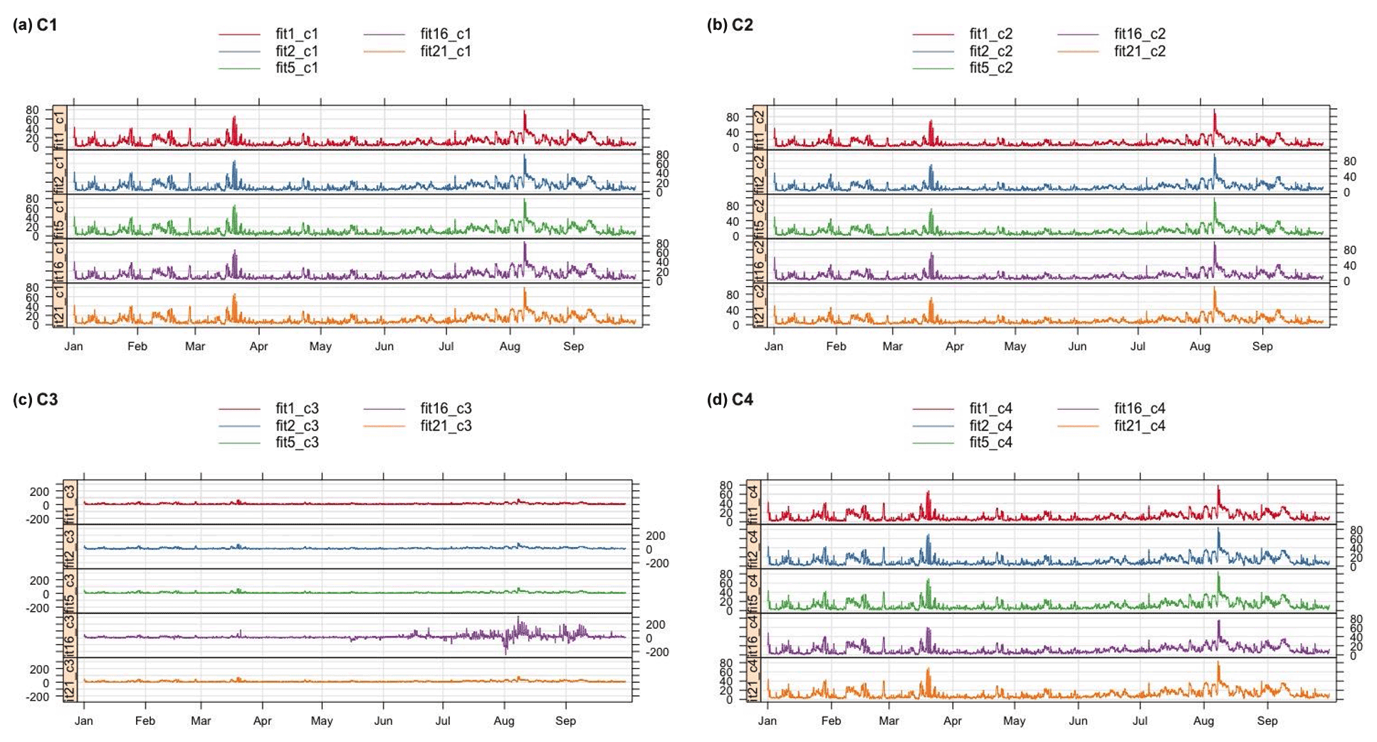
Figure 4Time series of the different PM2.5 corrected values for Models 1, 2, 5, 16, and 21 across corrections (a) C1, (b) C2, (c) C3, and (d) C4 for the Love My Air monitor CS1. Note that the scales are the same for C1, C2, and C4, but not for C3.
3.2 Evaluating sensitivity of the spatial and temporal trends of the low-cost sensor network to the method of calibration
The spatial and temporal RMSD values between corrected values generated from applying each of the 89 models using the four different correction approaches across all monitoring sites in the Love My Air network are displayed in Figs. 5 and 6, respectively. There is a larger temporal variation (max 32.79 µg m−3) in comparison to spatial variations displayed across corrections (max 11.95 µg m−3). Model 16 generated using the C3 correction has the greatest spatial and temporal RMSD in comparison with all other models. Models generated using the C3 and C4 corrections displayed the greatest spatial and temporal RMSD vis-a-vis C1 and C2.
Figures S14–S17 display spatial RMSD values between all models corresponding to corrections C1–C4, respectively, to allow for a zoomed-in view of the impact of the different model forms for the four corrections. Similarly, Figs. S18–S21 display temporal RMSD values between all models corresponding to corrections C1–C4, respectively. Across all models, the temporal RMSD between models is greater than the spatial RMSD.
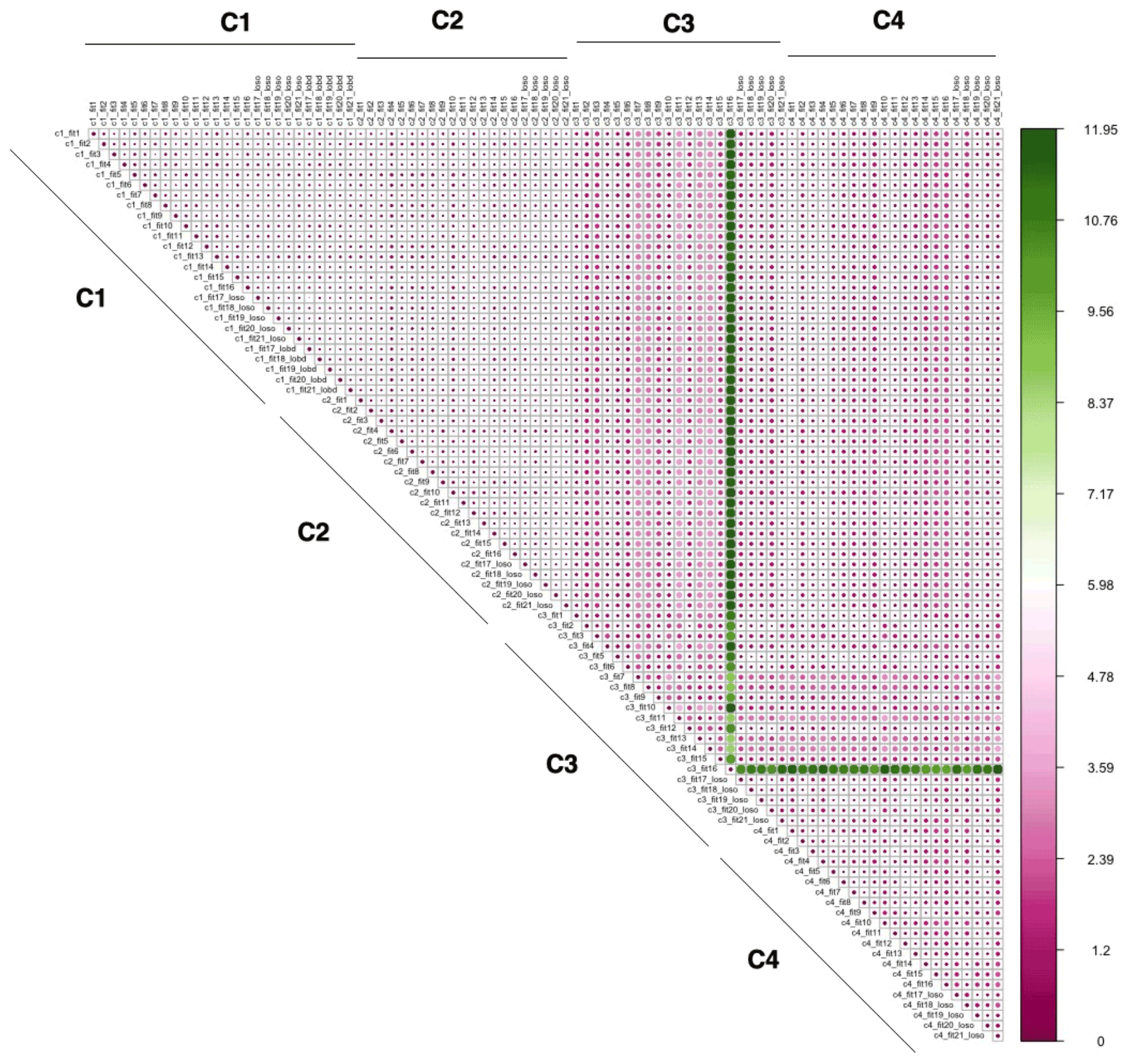
Figure 5Spatial RMSD (µg m−3) calculated using the method detailed in Sect. 2.3.5 from applying each of the 89 calibration models using the four different correction approaches to all monitoring sites in the Love My Air network.
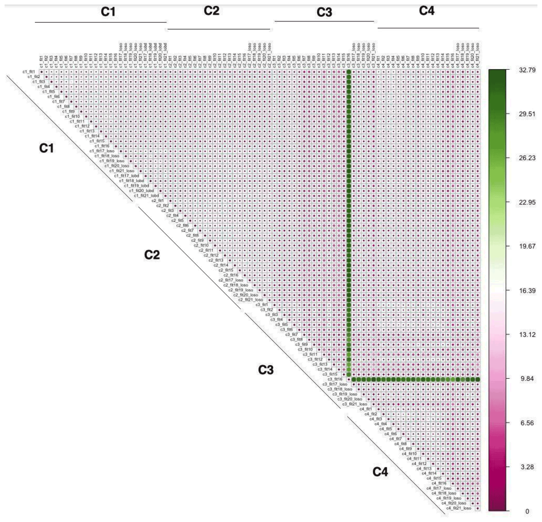
Figure 6Temporal RMSD (µg m−3) calculated using the method detailed in Sect. 2.3.5 from applying each of the 89 calibration models using the four different correction approaches to all monitoring sites in the Love My Air network.
The distribution of uncertainty and the NR in hourly calibrated measurements over the 89 models by monitor are displayed in Fig. 7. Overall, there are small differences in uncertainties and NR of the calibrated measurements across sites. The average NR and uncertainty across all sites are 1.554 (median: 0.9768) and 0.044 (median: 0.033), respectively. We note that, although the uncertainties in the data are small, the average normalized range tends to be quite large.

Figure 7Distribution of (a) uncertainty and (b) normalized range (NR) in hourly calibrated measurements across all 89 calibration models at each site using the methodology described in Sect. 2.3.5.
3.3 Evaluating the sensitivity of hotspot detection across the network of sensors to the calibration method
Mean (95 % CI) PM2.5 concentrations across the 89 different calibration models listed in Tables 1 and 2 at each Love My Air site for the duration of the experiment (1 January–30 September 2021) are displayed in Fig. S22. Due to overlap between the different calibrated measurements across sites, the ranking of sites based on pollutant concentrations is dependent on the calibration model used.
Every hour, we ranked the different monitors for each of the 89 different calibration models in order to evaluate how sensitive pollution hotspots were to the calibration model used. We found that there were, on average, 4.4 (median =5) sensors that were ranked most polluted. When this calculation was repeated using daily averaged calibrated data, there were, on average, 2.5 (median =2) sensors that were ranked the most polluted. The corresponding value for weekly calibrated data was 2.4 (median =1) and for monthly data was 3 (median =3) (Fig. 8).
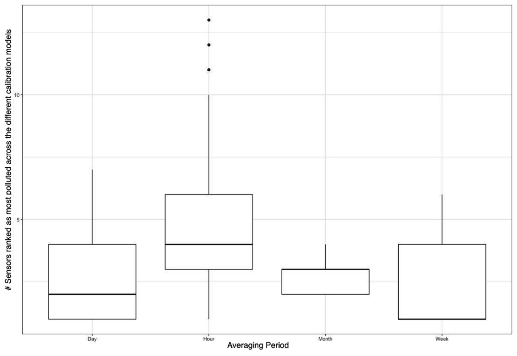
Figure 8Variation in the number of sites that were ranked as “most polluted” across the 89 different calibration models for different time-averaging periods displayed using box plots.
3.4 Supplementary analysis: evaluating transferability of calibration models developed in different pollution regimes
When we evaluated how well the models performed at high PM2.5 concentrations (>30 µg m−3) versus lower concentrations (≤30 µg m−3), we found that multivariate regression models generated using the C1 correction did not perform well in capturing peaks in PM2.5 concentrations (normalized RMSE >25 %) (Tables S3 and S4).
Multivariate regression models generated using the C2 correction performed better than those generated using C1 (normalized RMSE ∼ 20 %–25 %). Machine learning models generated using both C1 and C2 corrections captured PM2.5 peaks well (C1: normalized RMSE ∼ 10 %–25 %, C2: normalized RMSE ∼ 10 %–20 %). Specifically, the C2 RF model (Model 21) yielded the lowest RMSE values (4.180 µg m−3, normalized RMSE: 9.8 %) of all models considered. The performance of models generated using C1 and C2 corrections in the low-concentration regime was the same as that over the entire dataset. This is because most measurements made were <30 µg m−3.
Models generated using C3 and C4 had the worst performance in both concentration regimes and yielded poorer agreement with reference measurements than even the uncorrected measurements. As in the case with the entire dataset, more complex multivariate regression models and machine learning models generated using C3 and C4 performed worse than more simple models in both PM2.5 concentration intervals (Tables S3 and S4).
3.5 Supplementary analysis: evaluating transferability of calibration models developed across different time aggregation intervals
We then evaluated how well the models generated using C1, C2, C3, and C4 corrections performed when applied to minute-level LCS data at co-located sites (Tables S5 and S6). We found that the machine learning models generated using C1 and C2 improved the performance of the LCS. Model 21 (CV = LOSO) generated using C1 yielded an RMSE of 15.482 µg m−3 compared to 16.409 µg m−3 obtained from the uncorrected measurements.
The more complex multivariate regression models yielded a significantly worse performance across all corrections. (Model 16 generated using C1 yielded an RMSE of 41.795 µg m−3). As in the case with the hourly averaged measurements, using correction C1, LOBD CV instead of LOSO for the machine learning models resulted in better model performance, except for Model 21. Few models generated using C3 and C4 resulted in improved performance when applied to the minute-level measurements (Tables S5 and S6).
In our analysis of how transferable the correction models developed at the Love My Air co-location sites are to the rest of the network, we found that, for C1 (corrections developed on the entire co-location dataset) and C2 (on-the-fly corrections), more complex model forms yielded better predictions (higher R, lower RMSE) at the co-located sites. This is likely because the machine learning models were best able to capture complex, non-linear relationships between the LCS measurements, meteorological parameters, and reference data when conditions at the co-location sites were representative of that of the rest of the network. Model 21, which included additional covariates intended to capture periodicities in the data, such as seasonality, yielded the best performance, suggesting that, in this study, the relationship between LCS measurements and reference data varies over time. One possible reason for this could be the impact of changing aerosol composition in time, which has been shown to impact the LCS calibration function (Malings et al., 2020).
When examining the short term, C3 (corrections developed on two weeks of co-located data at the start of the experiment) and C4 (corrections developed on two weeks of co-located data in January and two weeks of co-located data in a May) corrections, we found that, although these corrections appeared to significantly improve LCS measurements during the time period of model development (Table S2), when transferred to the entire time period of operation, they did not perform well (Table 2). Many of the models, especially the more complex multivariate regression models, performed significantly worse than even the uncorrected measurements. This result indicates that calibration models generated during short time periods, even if the time periods correspond to different seasons, may not necessarily transfer well to other times, likely because conditions during co-location (aerosol-type, meteorology) are not representative of that of network operating conditions. Our results suggest the need for statistical calibration models to be developed over longer time periods that better capture different LCS operating conditions. However, for C3 and C4, we did find models that relied on nonlinear formulations of RH, which serve as proxies for hygroscopic growth, yielded the best performance as compared to more complex models (Table 2). This suggests that physics-based calibrations are potentially an alternative approach, especially when relying on short co-location periods, and need to be explored further.
When evaluating how transferable different calibration models were to the rest of the network, we found that, for C1 and C2, more complex models that appeared to perform well at the co-location sites did not necessarily transfer best to the rest of the network. Specifically, when we tested these models on a co-located site that was left out when generating the calibration models, we found that some of the more complex models using the C2 correction yielded a significantly worse performance at some test sites (Fig. 3). If the corrected data were going to be used to make site-specific decisions, then such corrections would lead to important errors. For C3 and C4, we observed a large distribution of RMSE values across sites. For several of the more complex models developed using C3 and C4 corrections, the RMSE values at some left-out sites were larger than observed for the uncorrected data, suggesting that certain calibration models could result in even more error-prone data than using uncorrected measurements. As the meteorological parameters for the duration of the C3 and C4 co-locations are not representative of overall operating conditions of the network, it is likely that the more complex models were overfit to conditions during the co-location, leading to them not performing well over the network operations.
For C1 and C2, we found that there were no significant differences in the distribution of the performance metric RMSE of corrected measurements from simpler models in comparison to those derived from more complex corrections at test sites (Fig. 3). For C3 and C4, we found significant differences in the distribution of RMSE across test sites, which indicates that these models are likely site specific and not easily transferable to other sites in the network. This suggests that less complex models might be preferred when short-term co-locations are carried out for sensor calibration, especially when conditions during the short-term co-location are not representative of that of the network.
We found that the temporal RMSD (Fig. 6) was greater than the spatial RMSD (Fig. 5) for the ensemble of corrected measurements developed by applying the 89 different calibration models to the Love My Air network. One of the reasons this may be the case is that PM2.5 concentrations across the different Love My Air sites in Denver are highly correlated (Fig. S5), indicating that the contribution of local sources to PM2.5 concentrations in the Denver neighborhoods in which Love My Air was deployed is small. Due to the low variability in PM2.5 concentrations across sites, it makes sense that the variations in the corrected PM2.5 concentrations will be seen in time rather than space. The largest pairwise temporal RMSD were all seen between corrections derived from complex models using the C3 correction.
Finally, we observed that the uncertainty in PM2.5 concentrations across the ensemble of 89 calibration models (Fig. 7) was consistently small for the Love My Air Denver network. The normalized range in the corrected measurements, on the other hand, was large; however, the uncertainty (95 % CI) in the corrected measurements fall within a relatively small interval. The average normalized range tends to be quite large, likely due to outlier corrected values produced from some of the more complex models evaluated using the C3 and C4 corrections. Thus, deciding which calibration model to pick has important consequences for decision makers when using data from this network.
Our findings reinforce the idea that evaluating calibration models at all co-location sites using overall metrics like RMSE should not be seen as the only or the best way to determine how to calibrate a network of LCS. Instead, approaches like the ones we have demonstrated and metrics like the ones we have proposed should be used to evaluate calibration transferability.
We found that the detection of the “most polluted” site in the Love My Air network (an important use case of LCS networks) was dependent on the calibration model used on the network. We also found that, for the Love My Air network, the detection of the most polluted site was sensitive to the duration of time averaging of the corrected measurements (Fig. 8). Hotspot detection was most robust using weekly averaged measurements. A possible reason for this is that temporal variations in PM2.5 in Denver varied primarily on a weekly scale, and therefore analysis conducted using weekly values resulted in the most robust results. Such an analysis thus provides guidance on the most useful temporal scale for decision making related to evaluating hotspots in the Denver network.
In supplementary analyses, when we evaluated the sensitivity of other LCS use cases to the calibration model applied, such as tracking high pollution concentrations during fire or smoke events, we found that different models yielded different performance results in different pollution regimens. Machine learning models developed using C1 and models developed using C2 were better than multivariate regression models generated using C1 at capturing peaks in pollution (>30 µg m−3). All models using C3 and C4 yielded poor performance results in tracking high pollution events (Tables S3 and S4). This is likely because PM2.5 concentrations during the C3 and C4 co-location tended to be low. The calibration model developed thus did not transfer well to other concentrations. When evaluating how well the calibration models developed using hourly aggregated measurements translated to high-resolution minute-level data (Tables S5 and S6), we observed that machine learning models generated using C1 and C2 improved the LCS measurements. More complex multivariate regression models performed poorly. All C3 and C4 models also performed poorly. This suggests that caution needs to be exercised when transferring models developed at a particular timescale to another. Note that, in this paper, because pollution concentrations did not show much spatial variation, we focus on evaluating transferability across timescales only.
In summary, this paper makes the case that it is not enough to evaluate calibration models based on metrics of performance at co-located sites, alone. We need to do the following:
-
Determine how well calibration adjustments can be transferred to other locations. Specifically, although we found that, in Denver, some calibration models performed well at co-location sites, the models could result in large errors at specific sites that would create difficulties for site-specific decision making.
-
Examine how well calibration adjustments can be transferred to other time periods. In this study, we found that models developed using the short-term C3 and C4 corrections were not transferable to other time periods, because the conditions during the co-location were not representative of broader operating conditions in the network.
-
Use a variety of approaches to quantify transferability of calibration models in the overall network (e.g., with spatiotemporal correlations and RMSD). The metrics proposed in this paper to evaluate model transferability can be used in other networks.
-
Investigate how adopting a certain timescale for averaging measurements could mitigate the uncertainty induced by the calibration process for specific use cases. Namely, we found that in the Love My Air network, hotspot identification was more robust when using daily averaged data than hourly averaged data. Our analyses also revealed which models performed best when needing to transfer the calibration model developed using hourly averaged data to higher-resolution data and which models best captured peaks in pollution during fire or smoke events.
In this work, the Love My Air network under consideration is located over a fairly small area in a single city. In this network, for the time period considered, PM2.5 seems to be mainly a regional pollutant, and the contribution of local sources is small. More work needs to be done to evaluate model transferability in networks in other settings. Concerns about model transferability are likely to be even more pressing when thinking about larger networks that span different cities and should be considered in future research. In this study, we present a first attempt to demonstrate the importance of considering the transferability of calibration models. In future work, we also aim to explore the physical factors that drive concerns about transferability to generalize our findings more broadly.
The code is available on reasonable request.
The data from the Love My Air air quality monitoring network used in this study can be obtained by contacting the Love My Air Program (https://www.denvergov.org/Government/Agencies-Departments-Offices/Agencies-Departments-Offices-Directory/Public-Health-Environment/Environmental-Quality/Air-Quality/Love-My-Air, Denver, 2022).
The supplement related to this article is available online at: https://doi.org/10.5194/amt-15-6309-2022-supplement.
PD conceptualized the study, developed the methodology, carried out the analysis, and wrote the first draft. PD and BC obtained funding for this study. BC produced Fig. 1. All authors helped in refining the methodology and editing the draft.
The contact author has declared that none of the authors has any competing interests.
Publisher’s note: Copernicus Publications remains neutral with regard to jurisdictional claims in published maps and institutional affiliations.
Priyanka deSouza and Ben Crawford gratefully acknowledge a CU Denver Presidential Initiative grant that supported their work. The authors are grateful to the Love My Air team for setting up and maintaining the Love My Air network. The authors are also grateful to Carl Malings for the useful comments
This paper was edited by Albert Presto and reviewed by two anonymous referees.
Anderson, G. B. and Peng, R. D.: weathermetrics: Functions to convert between weather metrics (R package), http://cran.r-project.org/web/packages/weathermetrics/index.html (last access: 26 October 2022), 2012.
Apte, J. S., Messier, K. P., Gani, S., Brauer, M., Kirchstetter, T. W., Lunden, M. M., Marshall, J. D., Portier, C. J., Vermeulen, R. C. H., and Hamburg, S. P.: High-Resolution Air Pollution Mapping with Google Street View Cars: Exploiting Big Data, Environ. Sci. Technol., 51, 6999–7008, https://doi.org/10.1021/acs.est.7b00891, 2017.
Barkjohn, K. K., Gantt, B., and Clements, A. L.: Development and application of a United States-wide correction for PM2.5 data collected with the PurpleAir sensor, Atmos. Meas. Tech., 14, 4617–4637, https://doi.org/10.5194/amt-14-4617-2021, 2021.
Bean, J. K.: Evaluation methods for low-cost particulate matter sensors, Atmos. Meas. Tech., 14, 7369–7379, https://doi.org/10.5194/amt-14-7369-2021, 2021.
Bi, J., Wildani, A., Chang, H. H., and Liu, Y.: Incorporating Low-Cost Sensor Measurements into High-Resolution PM2.5 Modeling at a Large Spatial Scale, Environ. Sci. Technol., 54, 2152–2162, https://doi.org/10.1021/acs.est.9b06046, 2020.
Brantley, H. L., Hagler, G. S. W., Herndon, S. C., Massoli, P., Bergin, M. H., and Russell, A. G.: Characterization of Spatial Air Pollution Patterns Near a Large Railyard Area in Atlanta, Georgia, Int. J. Env. Res. Pub. He., 16, 535, https://doi.org/10.3390/ijerph16040535, 2019.
Castell, N., Dauge, F. R., Schneider, P., Vogt, M., Lerner, U., Fishbain, B., Broday, D., and Bartonova, A.: Can commercial low-cost sensor platforms contribute to air quality monitoring and exposure estimates?, Environ. Int., 99, 293–302, https://doi.org/10.1016/j.envint.2016.12.007, 2017.
Clements, A. L., Griswold, W. G., RS, A., Johnston, J. E., Herting, M. M., Thorson, J., Collier-Oxandale, A., and Hannigan, M.: Low-Cost Air Quality Monitoring Tools: From Research to Practice (A Workshop Summary), Sensors, 17, 2478, https://doi.org/10.3390/s17112478, 2017.
Considine, E. M., Reid, C. E., Ogletree, M. R., and Dye, T.: Improving accuracy of air pollution exposure measurements: Statistical correction of a municipal low-cost airborne particulate matter sensor network, Environ. Pollut., 268, 115833, https://doi.org/10.1016/j.envpol.2020.115833, 2021.
Crawford, B., Hagan, D. H., Grossman, I., Cole, E., Holland, L., Heald, C. L., and Kroll, J. H.: Mapping pollution exposure and chemistry during an extreme air quality event (the 2018 Kīlauea eruption) using a low-cost sensor network, P. Natl. Acad. Sci. USA, 118, e2025540118, https://doi.org/10.1073/pnas.2025540118, 2021.
Crilley, L. R., Shaw, M., Pound, R., Kramer, L. J., Price, R., Young, S., Lewis, A. C., and Pope, F. D.: Evaluation of a low-cost optical particle counter (Alphasense OPC-N2) for ambient air monitoring, Atmos. Meas. Tech., 11, 709–720, https://doi.org/10.5194/amt-11-709-2018, 2018.
Denver: Love My Air, https://www.denvergov.org/Government/ Agencies-Departments-Offices/Agencies-Departments-Offices-Directory/Public-Health-Environment/Environmental-Quality/Air-Quality/Love-My-Air, last access: 22 October 2022.
deSouza, P. and Kinney, P. L.: On the distribution of low-cost PM2.5 sensors in the US: demographic and air quality associations, J. Expo. Sci. Env. Epid., 31, 514–524, https://doi.org/10.1038/s41370-021-00328-2, 2021.
deSouza, P., Anjomshoaa, A., Duarte, F., Kahn, R., Kumar, P., and Ratti, C.: Air quality monitoring using mobile low-cost sensors mounted on trash-trucks: Methods development and lessons learned, Sustain. Cities Soc., 60, 102239, https://doi.org/10.1016/j.scs.2020.102239, 2020a.
deSouza, P., Lu, R., Kinney, P., and Zheng, S.: Exposures to multiple air pollutants while commuting: Evidence from Zhengzhou, China, Atmos. Environ., 247, 118168, https://doi.org/10.1016/j.atmosenv.2020.118168, 2020b.
deSouza, P. N.: Key Concerns and Drivers of Low-Cost Air Quality Sensor Use, Sustainability, 14, 584, https://doi.org/10.3390/su14010584, 2022.
deSouza, P. N., Dey, S., Mwenda, K. M., Kim, R., Subramanian, S. V., and Kinney, P. L.: Robust relationship between ambient air pollution and infant mortality in India, Sci. Total Environ., 815, 152755, https://doi.org/10.1016/j.scitotenv.2021.152755, 2022.
Giordano, M. R., Malings, C., Pandis, S. N., Presto, A. A., McNeill, V. F., Westervelt, D. M., Beekmann, M., and Subramanian, R.: From low-cost sensors to high-quality data: A summary of challenges and best practices for effectively calibrating low-cost particulate matter mass sensors, J. Aerosol Sci., 158, 105833, https://doi.org/10.1016/j.jaerosci.2021.105833, 2021.
Hagler, G. S. W., Williams, R., Papapostolou, V., and Polidori, A.: Air Quality Sensors and Data Adjustment Algorithms: When Is It No Longer a Measurement?, Environ. Sci. Technol., 52, 5530–5531, https://doi.org/10.1021/acs.est.8b01826, 2018.
Holstius, D. M., Pillarisetti, A., Smith, K. R., and Seto, E.: Field calibrations of a low-cost aerosol sensor at a regulatory monitoring site in California, Atmos. Meas. Tech., 7, 1121–1131, https://doi.org/10.5194/amt-7-1121-2014, 2014.
Jin, X., Fiore, A. M., Civerolo, K., Bi, J., Liu, Y., Donkelaar, A. van, Martin, R. V., Al-Hamdan, M., Zhang, Y., Insaf, T. Z., Kioumourtzoglou, M.-A., He, M. Z., and Kinney, P. L.: Comparison of multiple PM2.5 exposure products for estimating health benefits of emission controls over New York State, USA, Environ. Res. Lett., 14, 084023, https://doi.org/10.1088/1748-9326/ab2dcb, 2019.
Kim, K.-H., Kabir, E., and Kabir, S.: A review on the human health impact of airborne particulate matter, Environ. Int., 74, 136–143, https://doi.org/10.1016/j.envint.2014.10.005, 2015.
Kuhn, M., Wing, J., Weston, S., Williams, A., Keefer, C., Engelhardt, A., Cooper, T., Mayer, Z., Kenkel, B., and R Core Team: Building predictive models in R using the caret package, R J., 223, 28, 1–26, 2020.
Kumar, P., Morawska, L., Martani, C., Biskos, G., Neophytou, M., Di Sabatino, S., Bell, M., Norford, L., and Britter, R.: The rise of low-cost sensing for managing air pollution in cities, Environ. Int., 75, 199–205, https://doi.org/10.1016/j.envint.2014.11.019, 2015.
Liang, L.: Calibrating low-cost sensors for ambient air monitoring: Techniques, trends, and challenges, Environ. Res., 197, 111163, https://doi.org/10.1016/j.envres.2021.111163, 2021.
Magi, B. I., Cupini, C., Francis, J., Green, M., and Hauser, C.: Evaluation of PM2.5 measured in an urban setting using a low-cost optical particle counter and a Federal Equivalent Method Beta Attenuation Monitor, Aerosol Sci. Technol., 54, 147–159, https://doi.org/10.1080/02786826.2019.1619915, 2020.
Malings, C., Tanzer, R., Hauryliuk, A., Saha, P. K., Robinson, A. L., Presto, A. A., and Subramanian, R.: Fine particle mass monitoring with low-cost sensors: Corrections and long-term performance evaluation, Aerosol Sci. Technol., 54, 160–174, https://doi.org/10.1080/02786826.2019.1623863, 2020.
Morawska, L., Thai, P. K., Liu, X., Asumadu-Sakyi, A., Ayoko, G., Bartonova, A., Bedini, A., Chai, F., Christensen, B., Dunbabin, M., Gao, J., Hagler, G. S. W., Jayaratne, R., Kumar, P., Lau, A. K. H., Louie, P. K. K., Mazaheri, M., Ning, Z., Motta, N., Mullins, B., Rahman, M. M., Ristovski, Z., Shafiei, M., Tjondronegoro, D., Westerdahl, D., and Williams, R.: Applications of low-cost sensing technologies for air quality monitoring and exposure assessment: How far have they gone?, Environ. Int., 116, 286–299, https://doi.org/10.1016/j.envint.2018.04.018, 2018.
Nilson, B., Jackson, P. L., Schiller, C. L., and Parsons, M. T.: Development and evaluation of correction models for a low-cost fine particulate matter monitor, Atmos. Meas. Tech., 15, 3315–3328, https://doi.org/10.5194/amt-2021-425, 2022.
Singh, A., Ng'ang'a, D., Gatari, M. J., Kidane, A. W., Alemu, Z. A., Derrick, N., Webster, M. J., Bartington, S. E., Thomas, G. N., Avis, W., and Pope, F. D.: Air quality assessment in three East African cities using calibrated low-cost sensors with a focus on road-based hotspots, Environ. Res. Commun., 3, 075007, https://doi.org/10.1088/2515-7620/ac0e0a, 2021.
Snyder, E. G., Watkins, T. H., Solomon, P. A., Thoma, E. D., Williams, R. W., Hagler, G. S. W., Shelow, D., Hindin, D. A., Kilaru, V. J., and Preuss, P. W.: The Changing Paradigm of Air Pollution Monitoring, Environ. Sci. Technol., 47, 11369–11377, https://doi.org/10.1021/es4022602, 2013.
Health Effects Institute: State of Global Air 2020, https://www.stateofglobalair.org/ (last access: 26 October 2022), 2020.
Van der Laan, M. J., Polley, E. C., and Hubbard, A. E.: Super learner, Stat. Appl. Genet. Mo. B., 6, 25, https://doi.org/10.2202/1544-6115.1309, 2007.
West, S. E., Buker, P., Ashmore, M., Njoroge, G., Welden, N., Muhoza, C., Osano, P., Makau, J., Njoroge, P., and Apondo, W.: Particulate matter pollution in an informal settlement in Nairobi: Using citizen science to make the invisible visible, Appl. Geogr., 114, 102133, https://doi.org/10.1016/j.apgeog.2019.102133, 2020.
Williams, R., Kilaru, V., Snyder, E., Kaufman, A., Dye, T., Rutter, A., Russel, A., and Hafner, H.: Air Sensor Guidebook, US Environmental Protection Agency, Washington, DC, EPA/600/R-14/159 (NTIS PB2015-100610), https://cfpub.epa.gov/si/si_public_record_Report.cfm?Lab=NERL&dirEntryId=277996 (last access: 26 October 2022), 2014.
Zimmerman, N., Presto, A. A., Kumar, S. P. N., Gu, J., Hauryliuk, A., Robinson, E. S., Robinson, A. L., and R. Subramanian: A machine learning calibration model using random forests to improve sensor performance for lower-cost air quality monitoring, Atmos. Meas. Tech., 11, 291–313, https://doi.org/10.5194/amt-11-291-2018, 2018.
Zusman, M., Schumacher, C. S., Gassett, A. J., Spalt, E. W., Austin, E., Larson, T. V., Carvlin, G., Seto, E., Kaufman, J. D., and Sheppard, L.: Calibration of low-cost particulate matter sensors: Model development for a multi-city epidemiological study, Environ. Int., 134, 105329, https://doi.org/10.1016/j.envint.2019.105329, 2020.