The Chalmers Cloud Ice Climatology: retrieval implementation and validation

Ice clouds are a crucial component of the Earth's weather system, and their representation remains a principal challenge for current weather and climate models. Several past and future satellite missions were explicitly designed to provide observations offering new insights into cloud processes, but these specialized cloud sensors are limited in their spatial and temporal coverage. Geostationary satellites have been observing clouds for several decades and can ideally complement the sparse measurements from specialized cloud sensors. However, the geostationary observations that are continuously and globally available over the full observation record are restricted to a small number of wavelengths, which limits the information they can provide on clouds.

The Chalmers Cloud Ice Climatology (CCIC) is a novel cloud-property dataset that aims to provide an improved climate record of ice hydrometeor concentrations by applying state-of-the-art machine-learning techniques to retrieve ice cloud properties from globally gridded, single-channel geostationary observations that are readily available from 1980 onwards. CCIC offers a novel perspective on the record of geostationary IR observations by providing spatially and temporally continuous retrievals of the vertically integrated and vertically resolved concentrations of frozen hydrometeors, typically referred to as ice water path (IWP) and ice water content (IWC). In addition to that, CCIC provides 2D and 3D cloud masks and a 3D cloud classification.

A fully convolutional quantile regression neural network constitutes the core of the CCIC retrieval, providing probabilistic estimates of IWP and IWC. The network is trained against CloudSat retrievals using 3.5 years of global collocations. Assessed on a held-out test dataset, the CCIC-provided IWP and IWC estimates achieve correlations exceeding 0.7 and 0.6, respectively, and biases better than −5 % and −2 % demonstrating considerable skill in estimating both IWP and IWC. In addition, CCIC is extensively validated against both in situ and remote sensing measurements from two flight campaign series and a ground-based radar. The results of this independent validation confirm the ability of CCIC to retrieve IWP and IWC. CCIC thus ideally complements temporally and spatially more limited measurements from dedicated cloud sensors by providing spatially and temporally continuous estimates of ice cloud properties. The CCIC network and its associated software are made accessible to the scientific community.

1 Introduction

The representation of clouds and convection in weather and climate models is recognized as a critical factor limiting the accuracy of forecasts of future weather and climate (Bony et al., 2015; Brunet et al., 2010). Moreover, the latest decadal survey of the National Academy of Science (National Academies of Sciences, Engineering, and Medicine, 2018) identified the question “Why do convective storms, heavy precipitation, and clouds occur exactly when and where they do?” as a key scientific question for the upcoming decade.

Several upcoming satellite missions and sensors were designed to provide new observations to improve the understanding of cloud processes and their representation in numerical models. The EarthCARE mission (Illingworth et al., 2015) will continue the combined radar–lidar observations from CloudSat (Stephens et al., 2002) and CALIPSO (Winker et al., 2010) and be the first space-borne sensor to measure vertical velocities of hydrometeors. In a similar vein, the Investigation of Convective Updrafts (INCUS) and NASA's Atmosphere Observation System (AOS) will provide measurements of the evolution of convective storms by means of a constellation of space-borne radars. Furthermore, sub-millimeter wave observations from the upcoming Ice Cloud Imager (ICI) on board the next generation of European polar-orbiting operational weather satellites will improve space-borne measurements of ice hydrometeor concentrations (Eriksson et al., 2020) by providing observations at sub-millimeter wavelengths.

While these and other future satellite missions will provide crucial, novel observations to further the understanding of convection and clouds, it will take several years before these observations are available and the observational record is sufficiently extensive to derive reliable results. The study of cloud processes on seasonal to annual scales will therefore depend on existing observations for the foreseeable future. While a variety of cloud products have been produced using a range of different satellite observations, many of them come with significant limitations that restrict their ability to help with studies of storm evolution or validate numerical models. Most cloud products that are based on sensors in low earth orbit, such as the MODIS Cloud Properties product (Platnick et al., 2015; Foster et al., 2021), provide only a limited of number of observations per day and thus can provide only very limited information on the evolution of individual cloud systems. Similarly, products derived from single sensors either are typically restricted in their spatial coverage (e.g., CLAAS-3; Benas et al., 2023) or have very high revisit times (Stephens et al., 2002; Winker et al., 2010). Moreover, while considerable effort has been devoted to reconciling currently available cloud datasets (Stubenrauch et al., 2024), significant differences remain between them, particularly in estimates of column-integrated ice concentrations (Eliasson et al., 2011; Duncan and Eriksson, 2018).

More specifically, Duncan and Eriksson (2018) showed that estimates of the zonal mean ice water path, i.e., the column-integrated concentration of frozen ice hydrometeors, differ by up to a factor of 5 between currently available datasets. The principal reasons for these discrepancies are differences in the sensitivity of the underlying sensors to ice particles of different sizes and uncertain assumptions on the microphysical properties of the observed clouds. Moreover, it is not always clearly defined whether the estimates provided by a product include all frozen hydrometeors or are limited to either suspended or precipitating particles.

Of the currently available cloud datasets providing global estimates of the ice water path, those derived from combined radar–lidar observations from the CloudSat and CALIOP satellites have to be considered the most accurate due to their ability to resolve the vertical structure of clouds and the combination of active measurements at microwave, IR, and visible wavelengths. However, due to the thin swath of these observations, their revisit time is on the order of a few weeks. Moreover, due to a technical failure, observations have been limited to daytime measurements since April 2011, and day- and nighttime measurements are only available between 2006 and 2011. Although global estimates of water paths are also provided by the MODIS, ISCCP-H series (Young et al., 2018), and PATMOS-x (Foster et al., 2023) products, which can be used to estimate the ice water path using provided cloud-phase information, these estimates are all limited to daytime observations. Furthermore, we were not able to find validation results for the ice water path estimates provided by the MODIS, ISCCP-H, and PATMOS-x datasets, thus making it difficult for users to gauge their accuracy.

The Chalmers Cloud Ice Climatology (CCIC) aims to address the above-listed shortcomings of the observational record of satellite-derived ice water path estimates by using state-of-the-art neural-network-based retrieval techniques to retrieve ice water path from the full available record of geostationary IR observations. The CCIC retrieval is trained to reproduce, and is thus calibrated to, combined radar–lidar estimates of frozen hydrometeor concentrations from the A-Train. CCIC provides estimates of the column-integrated concentrations of both suspended and precipitating ice particles, which we will refer to as the total ice water path (TIWP) to stress the inclusion of all ice particles in the estimates. CCIC is motivated by the findings from Pfreundschuh et al. (2022c) and Amell et al. (2022), which showed that neural-network-based retrievals that leverage the spatial structure of satellite observations can achieve considerably higher accuracy than traditional retrieval methods. CCIC provides estimates of TIWP and several other cloud properties from a single IR window channel centered around 11 µm. Although these observations primarily provide information on the temperature of the atmosphere at the cloud top, the 11 µm channel provides the best availability among currently available gridded geostationary observation datasets (Knapp et al., 2011) and thus allows producing a long time series of spatially and temporally continuous TIWP measurements albeit limited to latitudes within −60 to 60° N. The primary aim of CCIC is to provide an updated, comprehensive, extensively validated, and easily accessible record of TIWP estimates that can both provide context for more accurate but generally more sparse measurements from upcoming cloud sensors and serve for the validation of kilometer-scale models resolving convective storms (Prein et al., 2015).

In this preliminary article, we present the neural-network-based retrieval algorithm underpinning CCIC and validate it against independent measurements of hydrometeor concentrations. This work constitutes the first step towards producing an updated climate record of TIWP estimates, and we plan to follow this up with the production and publication of TIWP estimates for the full record of available geostationary IR observations.

The remainder of this article is organized as follows. Section 2 describes the dataset that was created for the training of the deep neural network used by CCIC and introduces the reference measurements used to validate the retrieval. Section 3 establishes the nominal accuracy of the retrieval by evaluating it on a held-out test dataset, while Sect. 4 assesses the retrieval against independent in situ and remote sensing measurements of hydrometeor concentrations. Finally, Sect. 5 discusses the validation results and potential applications of CCIC, and Sect. 6 summarizes the principal conclusions from this study.

2 Methods and data

The CCIC retrieval is based on a convolutional neural network (CNN) that leverages quantile regression (Pfreundschuh et al., 2018) to provide probabilistic estimates of TIWP as well as additional cloud properties. The following subsections describe the implementation and training of the neural-network-based retrieval. Following this, the independent measurements used to validate the CCIC retrieval are presented.

2.1 The CCIC retrieval

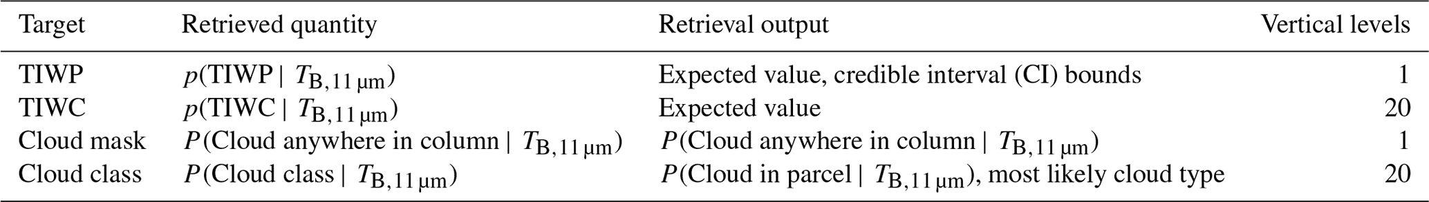
In order to allow the application of the retrieval to the extensive historical record of geostationary IR observations, CCIC was designed to use 11 µm IR brightness temperatures as the only retrieval input. The retrieval does not ingest any ancillary data to make the estimates independent from other datasets. As mentioned in the Introduction, TIWP constitutes the primary retrieval target of CCIC. However, it is accompanied by the vertically resolved concentration of ice hydrometeors, referred to as “total ice water content” (TIWC). Analogously to TIWP, the name TIWC was chosen to emphasize that the estimates of total mass of frozen hydrometeors are not restricted to a single species. Additional, secondary retrieval targets provided by CCIC are a vertically resolved and a vertically integrated cloud mask. Table 1 summarizes the CCIC retrieval targets.

Table 1 CCIC retrieval targets. CCIC provides probabilistic estimates of the cloud properties listed in this table. Due to storage limitations only the statistics listed under “Retrieval output” are actually retained as output. The cloud classification is based on the nine cloud classes from the CloudSat 2B-CLDCLASS product (no cloud; cirrus, Ci; altostratus, As; altocumulus, Ac; stratus, St; stratocumulus, Sc; cumulus, Cu; nimbostratus, Ns; and deep convection, DC).

2.1.1 Input data

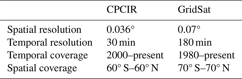
The CCIC retrieval ingests geostationary IR input data from two distinct datasets in order to maximize the spatiotemporal coverage and resolution of the CCIC data record. The first dataset is the GridSat-B1 product version 2 (GridSat; Knapp et al., 2011; Knapp and NOAA CDR Program, 2014), which covers the time from 1980 until the present at a temporal resolution of 3 h and a spatial resolution of 0.07°. The second dataset is the NOAA Climate Prediction Center globally merged IR product version 1 (CPCIR; Janowiak et al., 2001, 2017), which is available only from the year 2000, with some data from 1998, but offers higher temporal and spatial resolutions of 30 min and 0.036°, respectively. Both datasets provide merged and gridded IR brightness temperatures from the channels closest to 11 µm from the global constellation of historical and current geostationary meteorological satellites. Knapp et al. (2011) and references therein detail that both datasets are provided after an intersatellite normalization, i.e., viewing angle and parallax corrections, and GridSat, in addition, employs a temporal calibration against High-resolution Infrared Radiation Sounder (HIRS) near-11 µm channel data, targeting long historical analyses. The IR radiances are used as input to the CCIC network without discerning between the datasets. The characteristics of the two datasets are summarized in Table 2.

Table 2 Spatiotemporal resolution and coverage of the input data products.

2.1.2 Training data

The reference data for the CCIC retrieval targets are derived from two CloudSat products: the level 2 cloud scenario classification version R05 (2B-CLDCLASS; Sassen and Wang, 2008) and the level 2 CloudSat and CALIPSO ice cloud property version R05 (2C-ICE; Deng et al., 2010, 2013b, 2015). The 2B-CLDCLASS product assigns each CloudSat radar bin one of nine different cloud classes (Table 1). This choice of reference data over similar products, e.g., DARDAR-cloud (Delanoë and Hogan, 2010), which can be regarded as the alternative to 2C-ICE, was motivated by the 2C-ICE product yielding smaller biases against in situ measurements (Deng et al., 2013a). We acknowledge that the referenced validation study was performed using now-outdated versions of the retrievals; however, we were not able to find more recent validation studies involving these two products.

The 2B-CLDCLASS and 2C-ICE granules were both collocated with the input data and used to extract the following information for each profile: TIWP, TIWC, a horizontal cloud mask indicating the presence of a cloud anywhere in the vertical profile, and vertically resolved cloud classification following the 2B-CLDCLASS product. Although there is redundancy in these variables, as TIWC integrates into TIWP and the 2D cloud mask can, in principle, be derived from the vertically resolved cloud classification, they were kept separate.

Despite the vertical information in the 2B-CLDCLASS and 2C-ICE products being provided in bins of 240 m, the reference data were regridded to a uniform altitude grid with a vertical resolution of 1 km relative to the surface of the digital elevation model provided in these products. The cloud class profiles were downsampled by a factor of 4 by randomly picking one bin in contiguous sets of four 2B-CLDCLASS height bins, followed by nearest-neighbor interpolation to the target altitude level. The random subsampling was performed to retain the uncertainty introduced by the subsampling of the vertical resolution of the reference data. For the regridding of TIWC, the vertical profiles were first smoothed with a Gaussian filter with a full width at half maximum of approximately 1 km. Afterwards, the smoothed values were linearly interpolated to the target altitude levels. Finally, TIWC values were scaled to ensure that the regridded profiles integrate to the same value as the corresponding TIWP.

The vertically subsampled reference data were collocated with the input data by binning the profiles with respect to the input data grid and then randomly sampling one profile from the multiple profiles collocated with each input pixel. Randomly choosing a profile retains the uncertainty due to the coarser resolution of the input observations, which is required for this uncertainty to be included in the uncertainty estimates provided by the probabilistic regression retrieval. An additional representation of reference TIWP was prepared by taking the average per input-data pixel. This alternative representation was included as a sanity check. While retrievals of the footprint-averaged TIWP are consistent with those based on the randomly sampled profile in terms of the posterior mean, the predicted retrieval uncertainties will refer to the footprint-averaged reference data and thus exhibit statistics that vary with the footprint size of the observations. Since it provides essentially the same information as the randomly sampled TIWP, it is not discussed further here. For the temporal collocation, the reference data were assigned to the closest input data with a maximum difference of 15 min between the profile observation time and the reference time of the gridded IR data.

CloudSat measurements are available from mid-2006 onwards but are limited to daylight observations from April 2011 due to a battery anomaly (Nayak et al., 2012). Consequently and for simplicity, only CloudSat data before 2011 were considered in order to minimize the risk of introducing a diurnal bias. Data in 2010 were assigned to a held-out test set, and all data for the other 3.5 years were used for training, with collocations in the first day of each month allocated to a validation set that was used to monitor training progress.

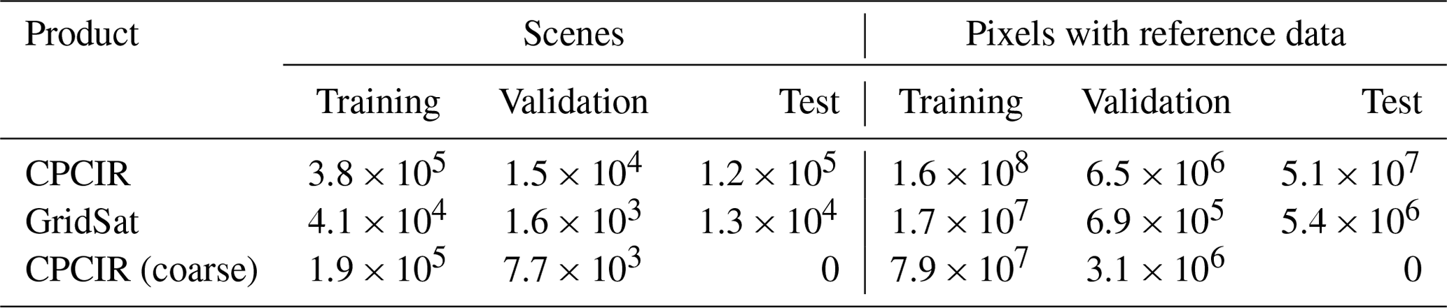
The collocated geostationary input observations and CloudSat–CALIPSO-based reference data are used to generate the training dataset, which consists of scenes with a horizontal extent of 384 × 384 px of input observations. The scene size of 384 px was chosen as it allows for the extraction of randomly rotated center crops of size 256 × 256 px, which is ultimately for training and inference. The extent of 256 × 256 px was chosen as it results in scenes exceeding 900 km in zonal and meridional extent and thus should contain information on the mesoscale and, to some extent, also the synoptic-scale context of the retrieval. Scenes are extracted by randomly selecting a pixel with valid reference data as the center point for the scene. Then, a random zonal shift of up to 50 px east or west is applied to the scene so that the relative position of the CloudSat swath within the scene is randomized. This process was repeated until all pixels with valid reference data were included in at least one training scene. Scenes with less than 20 % of valid reference data pixels were discarded. Figure 1 shows that there is a clear difference in the spatial distributions of the collocations between the two IR data products, which is a result of the fixed overpass times of CloudSat and the coarser temporal resolution of the GridSat data. An additional CPCIR training and validation dataset was prepared at a coarser resolution: the CPCIR data were preprocessed by subsampling every 2 px, thus approximately matching the GridSat resolution, and then processed in the same way as the other two datasets. This aimed to mitigate any potential underfit for GridSat given the imbalanced data. Table 3 shows the sizes of the training, validation, and test datasets. All codes required to generate the training datasets are made available through the code repository accompanying this article (Amell and Pfreundschuh, 2023).

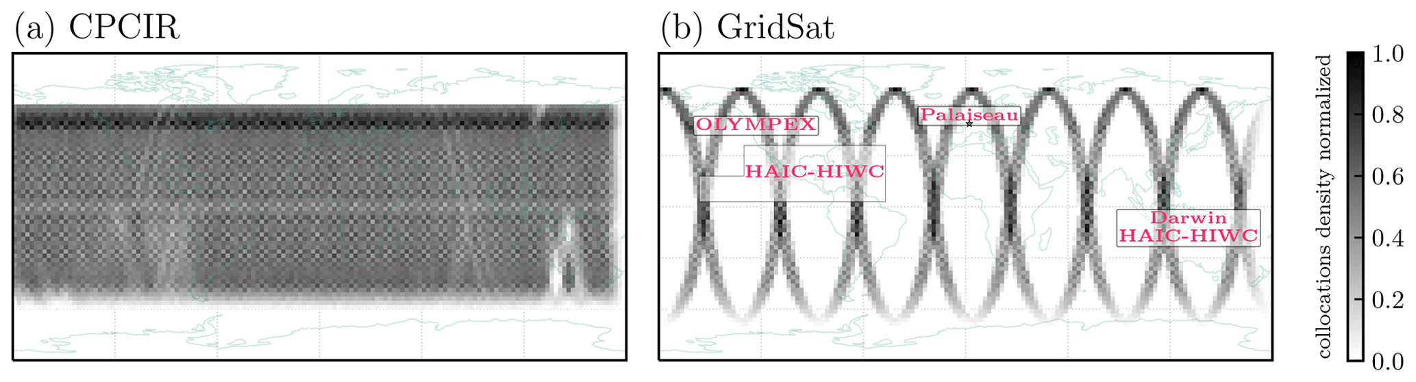
Figure 1 Spatial distributions of the pixels with valid reference values in the training set, binned on a 2.5° × 2.5° grid. Panel (b) also displays the approximate spatial coverage of three campaigns and the ground-based cloud radar site used in the validation of CCIC.

Table 3 Total number of scenes and pixels with valid profiles for each input dataset in the database.

The distributions of the target variables (Appendix A) show marginal differences when collocated with GridSat or CPCIR. It is assumed that these differences come from the available collocations for each product (see Fig. 1) and are deemed negligible. The distributions of both TIWP and TIWC are heavily right-skewed, spanning several orders of magnitude. Atmospheric states without ice masses are predominant, although nearly half of the pixels are cloudy; besides cloud-free scenarios, the three most frequent clouds in the training are altostratus, nimbostratus, and cirrus, in this order (Table A1).

2.1.3 Neural network architecture

Figure 2 illustrates the architecture of the CNN used for the CCIC retrieval. The model consists of convolutional encoder and decoder modules that are shared between all retrieval targets and a separate head for every retrieval target. The convolutional blocks used in the encoder and decoder of the CNN are similar to those of the ConvNeXt architecture (Liu et al., 2022) with layer normalization (Ba et al., 2016) arranged in an asymmetric encoder–decoder, U-net-like architecture (Ronneberger et al., 2015). The network heads each consist of several blocks of 1 × 1 convolutions, normalization layers, and activation functions, and they map the shared features extracted by the encoder and decoder to the output of each variable. The basic architecture is grounded in previous retrievals (Amell et al., 2022; Pfreundschuh et al., 2022c, a), and since it provides good results, no extensive tuning of the model architecture or hyperparameters was performed.

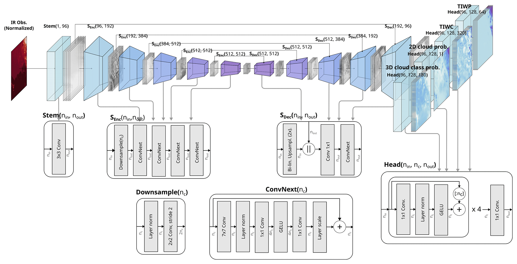
Figure 2 The artificial neural network used in CCIC. The input is the brightness temperatures T_B,11 µm normalized with $T_{\mathrm{B},\mathrm{11}\mathrm{\mu }\mathrm{m},min}$ = 170 K and $T_{\mathrm{B},\mathrm{11}\mathrm{\mu }\mathrm{m},max}$ = 310 K. The number of output neurons for each head matches the number of quantiles or classes needed for each variable. The network contains 4.3×10⁷ learnable parameters. Symbols: $\left|\right|$ is depthwise concatenation, [:n_c] is slicing and keeping the first n_c channels, and + is depthwise addition.

Because of the very limited information content of the input observations, the mapping from IR brightness temperatures to hydrometeor concentrations can be expected to exhibit significant retrieval uncertainty. The retrieval uncertainty, which is referred to in the machine-learning community as “aleatoric uncertainty”, can be quantified using quantile regression neural networks (QRNNs; Pfreundschuh et al., 2018), making the resulting retrieval equivalent to a traditional Bayesian retrieval. Since QRNNs provide a piecewise linear estimate of the cumulative distribution function (CDF) of the marginal distribution of every output variable, no assumptions are required regarding the functional form of the distributions. The approach can thus represent non-Gaussian retrieval uncertainties while simultaneously leveraging the predictive power of deep, convolutional neural networks.

2.1.4 Training

The CCIC retrieval was trained using multitask supervised learning; i.e., the losses from all retrieval targets were optimized simultaneously. Since the CCIC retrieval targets comprise both continuous and categorical variables, the network was trained to minimize a mixed loss, defined as the sum of the cross-entropy averages for the categorical variables and the multiple quantile regression loss averages used in QRNNs for the continuous output variables. No scaling was applied in the total loss function for the different targets. The loss functions for each class of variables are given by

$$\begin{array}{}\text{(1)}& {\mathcal{L}}_{\mathrm{categorical}}=-{\displaystyle \frac{\mathrm{1}}{N}}\sum _{i=\mathrm{1}}^N\log \left({\displaystyle \frac{\exp y_i^{\left(c\right)}}{{\sum }_{j=\mathrm{1}}^C\exp y_i^{\left(j\right)}}}\right)\end{array}$$

and

$$\begin{array}{}\text{(2)}& {\mathcal{L}}_{\mathrm{continuous}}={\displaystyle \frac{\mathrm{1}}{N\left|\mathcal{T}\right|}}\sum _{i=\mathrm{1}}^N\sum _{\mathit{\tau }\in \mathcal{T}}\left(x_i-{\widehat{x}}_i^{\left(\mathit{\tau }\right)}\right)\left(\mathit{\tau }-\mathbb{I}\left(x_i\le {\widehat{x}}_i^{\left(\mathit{\tau }\right)}\right)\right).\end{array}$$

Here, N indicates the number of reference values; $y_i^{\left(j\right)}$ the output value for class j, with class c being the reference class; 𝒯 a set of predefined quantiles and |T| its cardinality; x_i the reference value; ${\widehat{x}}_i^{\left(\mathit{\tau }\right)}$ the predicted quantile at level τ; and 𝕀 the indicator function.

The continuous variables TIWP and TIWC span over several orders of magnitude, where each order can be considered to contain significant information. The training applied the log-linear transform

$$\begin{array}{}\text{(3)}& f\left(x\right)=\log \left(x\right)\mathbb{I}(x<\mathrm{1})+(x-\mathrm{1})\mathbb{I}(x\ge \mathrm{1})\end{array}$$

on the reference values, with TIWP and TIWC expressed in kg m⁻² and g m⁻³, respectively, to address this challenge. Since the log transform is defined only for strictly positive values, TIWP and TIWC values below a clear-sky threshold t are replaced with random values from a log-uniform distribution in [a,b]: for TIWP (in kg m⁻²), $t={\mathrm{10}}^{-\mathrm{3}}$, $a={\mathrm{10}}^{-\mathrm{6}}$, and $b={\mathrm{10}}^{-\mathrm{4}}$; for TIWC (in g m⁻³), $t={\mathrm{10}}^{-\mathrm{7}}$, $a={\mathrm{10}}^{-\mathrm{10}}$, and $b={\mathrm{10}}^{-\mathrm{8}}$. This treatment of small and zero values ensures that the quantiles of the posterior distribution are well calibrated. Since the predicted quantiles are invariant to strictly monotonically increasing transformations, the transformation does not change the statistical properties of the resulting prediction.

The QRNN retrievals use different quantile levels for TIWP and TIWC. For TIWP, the network outputs a quantile-parameterized distribution (QPD) with 64 quantile levels, given by ${\mathcal{T}}_{\mathrm{TIWP}}=\left\{\mathrm{0.001},\mathrm{1}{\mathrm{\Delta }}_{\mathrm{TIWP}},\mathrm{2}{\mathrm{\Delta }}_{\mathrm{TIWP}},\mathrm{\dots },\mathrm{62}{\mathrm{\Delta }}_{\mathrm{TIWP}},\mathrm{0.999}\right\}$, where ${\mathrm{\Delta }}_{\mathrm{TIWP}}=\mathrm{1}/\mathrm{63}$. For TIWC, the QPD at each altitude level is given by the 16 quantile levels ${\mathcal{T}}_{\mathrm{TIWC}}=\left\{\mathrm{0.01},\mathrm{0.05},\mathrm{1}{\mathrm{\Delta }}_{\mathrm{TIWC}},\mathrm{2}{\mathrm{\Delta }}_{\mathrm{TIWC}},\mathrm{\dots },\mathrm{13}{\mathrm{\Delta }}_{\mathrm{TIWC}},\mathrm{0.95},\mathrm{0.99}\right\}$, with ${\mathrm{\Delta }}_{\mathrm{TIWC}}=\mathrm{1}/\mathrm{15}$. This arrangement of the quantile levels was found to produce better retrievals than strictly equally spaced levels. Any quantile between the levels 𝒯_TIWP or 𝒯_TIWC can be obtained with a linear interpolation of the QPD.

The CCIC neural network (NN) was trained on four NVIDIA Tesla V100 SXM2 32 GB GPUs for about 80 epochs using a cosine-annealing learning rate schedule (Loshchilov and Hutter, 2016), with one epoch taking about 280 min. Monitoring of the validation loss during training showed no overfitting, and the training losses converged. Missing pixels in the input are replaced by a constant special value, while missing reference data are masked out and simply ignored in the loss calculation. Random rotations and flips, followed by random cropping of the input image to 256 × 256 px, were used to augment the training data. Appendix B provides additional details on the training.

2.2 Validation data

The CCIC retrievals are trained to reproduce the data from the CloudSat 2B-CLDCLASS and 2C-ICE datasets, which are themselves derived from remote sensing observations. Since these datasets are used as the ground truth during training, their errors will be reproduced by CCIC. It is therefore essential to compare the CCIC results to independent and ideally more direct measurements of ice cloud properties. While the most direct measurements of frozen hydrometeors are arguably in situ measurements, these are inherently sparse and typically only provide estimates of the TIWC at a certain altitude in the atmosphere rather than the TIWP, which would require measuring ice hydrometeor concentrations over the full height of the atmosphere.

In addition to in situ measurements of frozen hydrometeors, we also make use of airborne and ground-based cloud radar observations. Although these measurements will likely be affected by similar uncertainties as the CloudSat-derived reference data, these data allow the validation of the CCIC retrieval outside the limited temporal sampling of the CloudSat observations. To compare radar observations from the different flight campaigns and the ground-based radar in a consistent manner, we have developed an additional retrieval that retrieves TIWC estimates from radar observations. These retrievals allow us to control the microphysical assumptions used in the retrieval, which constitute a major source of uncertainty in the resulting TIWC estimates. We run the retrieval for multiple assumed ice particle habits, and for each campaign we use the results that yield the best consistency with the in situ measurements. The implementation of the retrieval is described in detail in Appendix C.

2.2.1 HAIC-HIWC

A series of international field campaigns took place between January 2014 and August 2018 to collect in situ measurements of hydrometeors and other cloud properties: the High Altitude Ice Crystals (HAIC; Dezitter et al., 2013), the High Ice Water Content (HIWC; Strapp et al., 2016a), and the HIWC radar (Ratvasky et al., 2019) projects. These campaigns, referred to as HAIC-HIWC, involved measurements of deep convective systems, including tropical storms, using probes and radar instruments mounted on research aircraft. The hydrometeor total water content (TWC) was one of the properties measured with probes during these campaigns. This property directly correlates with the TIWC at low temperatures, which is where most of the measurements were performed.

The IKP-2 probe (Strapp et al., 2016b; Davison et al., 2016) was specifically developed to measure TWC in HAIC-HIWC. All openly available HAIC-HIWC TWC data measured with this probe were collocated with TIWC CCIC retrievals by averaging them in 4D bins, defined by the GridSat or CPCIR grid; 1 km altitude bins centered at the CCIC altitude levels; and 30 min temporal bins centered on the GridSat or CPCIR timestamps. Figure 3 presents the spatial coverage of the collocations obtained with this method.

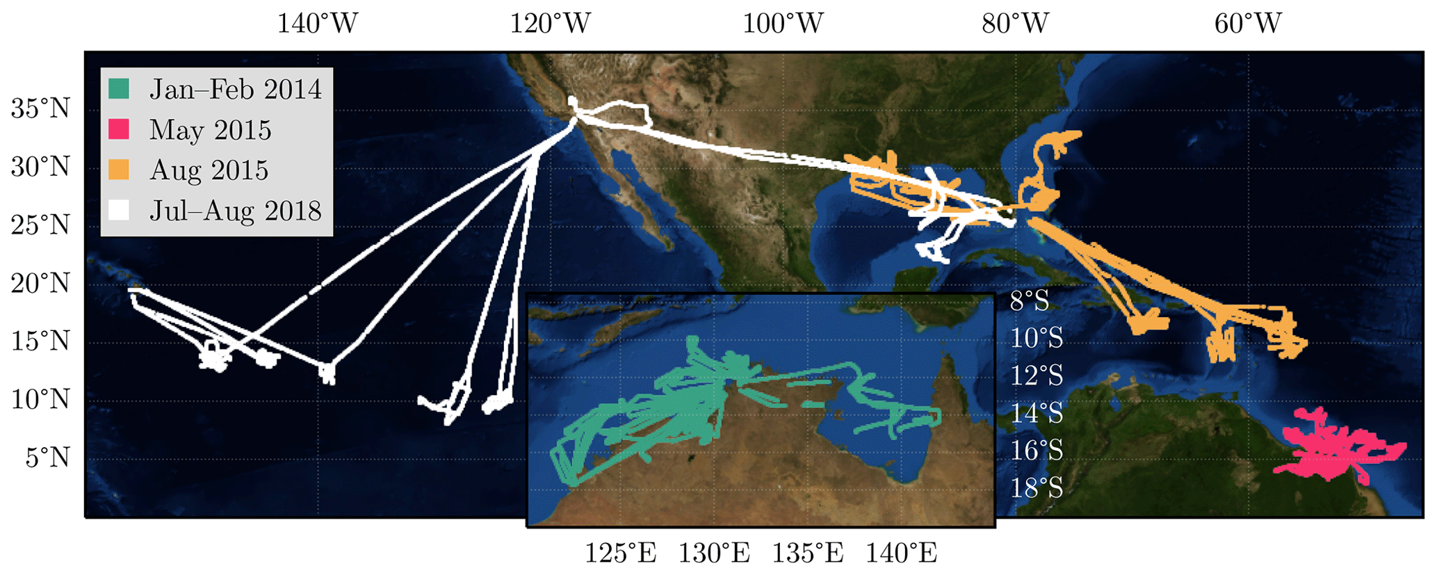
Figure 3 Spatial coverage of in situ measurements of TWC collected during the different HAIC-HIWC campaigns and collocated with CCIC retrievals. Flights during January and February 2014 were performed over Darwin, Australia, and the surrounding oceans. Flights during May 2015 were performed out of Cayenne, French Guyana. Flights during August 2015 were performed out of Fort Lauderdale, USA. Flights in August 2018 were based out of Fort Lauderdale, Palmdale on the west coast of the USA, and Kona in Hawaii. The map background is based on NASA Visible Earth imagery.

In addition to the in situ measurements collected during all flights of the HAIC-HIWC campaigns, the first campaign in Darwin, Australia, also included 95 GHz cloud radar measurements from the Radar Airborne System Tool for Atmosphere (RASTA) radar flown on board the Falcon 20 of the Service des Avions Français Instrumentés pour la Recherche en Environnement (SAFIRE) that are publicly available. Since these observations allow for a more complete characterization of the vertical structure of the observed clouds than the in situ measurements alone, they are used here as an additional source of validation data.

2.2.2 OLYMPEX

The Olympic Mountain Experiment (OLYMPEX; Houze et al., 2017) was carried out between late fall 2015 and early spring 2016 with the principal aim to investigate the effect of the Olympic mountains on precipitation. As part of the campaign, 94 GHz cloud radar observations were performed by the NASA Cloud Radar System (CRS; Li et al., 2004) on board the NASA ER-2 aircraft. In addition to this, in situ measurements of concentrations of frozen hydrometeors were performed by the University of North Dakota (UND) Cessna Citation aircraft.

We use both radar retrievals of TIWC from the NASA CRS radar as well as the in situ measurements from the UND Citation aircraft to validate the CCIC retrievals. The flight paths of the two aircraft are displayed in Fig. 4. The airborne measurements are collocated with CCIC retrievals by downsampling them to the spatial resolution of the CPCIR and GridSat observations following the method from Sect. 2.2.1.

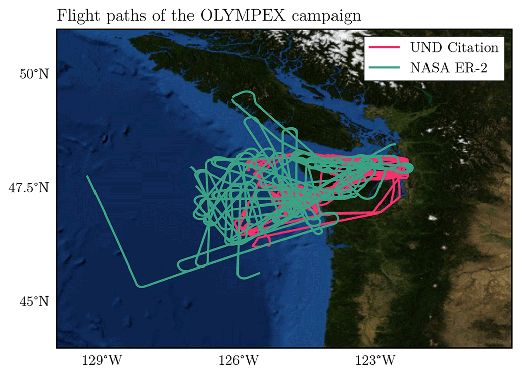
Figure 4 Flight paths of the UND Citation and NASA ER-2 aircraft during the OLYMPEX campaign over the Olympic Peninsula in the pacific northwest region of the USA. The map background is based on NASA Visible Earth imagery.

2.2.3 Cloudnet

The Aerosol, Clouds and Trace Gases Research Infrastructure (ACTRIS) Cloudnet data portal curates and provides access to ground-based remote sensing measurements of clouds. In contrast to flight campaigns, measurements from permanent, ground-based radars allow for the evaluation of CCIC over annual and seasonal timescales. For this study we use 1 year (2019) of radar measurements (Delanoë and Haeffelin, 2023) from the 95 GHz Bistatic Radar System for Atmospheric Studies (BASTA; Delanoë et al., 2016) from the site in Palaiseau, France. This Cloudnet site was chosen as it presented one of the most complete W-band cloud radar data records, in particular for 2019, for the latitudes covered by the CCIC retrievals.

3 Retrieval characterization

This section evaluates the accuracy of the CCIC retrieval against held-out test data derived from CloudSat observations.

3.1 Case study

To provide an overview of the capabilities and retrieval targets of CCIC, a case study of a midlatitude cyclone over the west coast of North America on 3 January 2019 is shown in Fig. 5. The case was chosen as it coincides with an overpass of CloudSat over the cyclone and thus allows the CCIC retrievals to be compared to the corresponding CloudSat measurements.

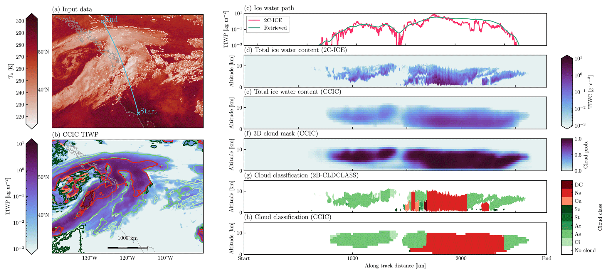
Figure 5 Retrieved and reference cloud properties from a CloudSat overpass over a midlatitude cyclone over the North American west coast on 3 January 2019. Panel (a) shows the CPCIR input observations. Panel (b) displays a map of the retrieved TIWP over the region as well as the dominant cloud type, which is defined as the most frequent non-clear cloud class (as defined in panels g and h) in the atmospheric column. Panel (c) shows the retrieved and reference TIWP along the CloudSat ground track marked by the blue line in panel (a). Panel (d) shows the TIWC from 2C-ICE along the CloudSat ground track. Panel (e) shows the corresponding retrieved TIWC. Panel (f) shows the retrieved 3D cloud mask. Panel (g) shows the cloud classification from the 2B-CLDCLASS product. Panel (h) shows the corresponding retrieved cloud classes.

Multiple cloud systems associated with fronts generated by the cyclone can be identified easily even in the IR observations. Compared to the IR input observations, the TIWP field exhibits significantly lower spatial variability, which is expected due to the smoothing effect of retrieval uncertainty on the retrieved posterior mean. Nonetheless, the overall spatial structure of the cloud systems is well reproduced in the TIWP field. It is notable that the distribution of TIWP within the clouds does not seem to exhibit a direct relationship with the corresponding brightness temperatures, indicating that the retrieval leverages spatial context to infer the retrieved TIWP. The contour lines showing the dominant cloud types clearly distinguish stratiform and convective regions of the observed cloud systems whose locations are consistent with the corresponding cloud-forming processes. In particular, stratiform clouds precede the leading warm front of the cyclone, whereas the convective clouds align with the cold and the occluded front. Interestingly, there is also a region of clouds in the southwest corner of the domain, where CCIC identifies St but retrieves no TIWP. This indicates that the retrieval also has some capability to distinguish the cloud phase.

Compared to the 2C-ICE retrieval along the CloudSat ground track, the CCIC TIWP retrieval exhibits less spatial variability but in general agrees with the 2C-ICE results. The reduced spatial resolution of the CCIC retrieval is even more apparent in the comparison of the retrieved TIWC. Nonetheless, to first order, the vertical structure of the cloud systems is reproduced correctly by the CCIC TIWC retrieval. In particular, the retrieval correctly reproduces the higher and less-dense clouds associated with the warm front and the lower and denser clouds of the occluded front.

The 3D cloud classification shows general agreement with the classes identified by 2B-CLDCLASS except for the region between 2100 and 2250 km along the transect. In this region, the full cloud system is classified as Ns, whereas CloudSat detects only a low-level Ns cloud covered by non-convective higher-level clouds. The inability of the CCIC retrievals to resolve the vertically heterogeneous structure of the clouds is certainly due to the limited information content in the IR input observations, which are primarily related to the cloud top temperature. However, an additional factor contributing to the differences between the cloud type classification of CloudSat and CCIC may be that the CCIC cloud-type estimates are from 21:00 UTC, while the CloudSat overpass was close to 21:15 UTC. Since the cloud system can be expected to move to the east, the relative position of CloudSat ground track at 21:15 UTC may be shifted slightly to the west, where the cloud cover is more heterogeneous. The cloud classification also fails to reproduce the small-scale variability in the CloudSat-based classification. Nonetheless, it is notable that the retrieval can reproduce much of the vertical structure of the observed cloud system.

3.2 Accuracy on test set

The following subsections quantitatively assess the accuracy of the CCIC retrieval on the independent test dataset, which consists of all CloudSat collocations from the year 2010.

3.2.1 Hydrometeor concentrations

Conditional distributions of the retrieved posterior mean of the TIWP conditioned on the reference TIWP value for the test dataset are shown in Fig. 6. The logarithmic shading of the distributions reveals a large spread around the diagonal indicative of considerable retrieval uncertainty. Nonetheless, with values of −3.33 % and −4.28 %, the overall retrieval biases are small and the correlations of 0.75 and 0.74 for the CPCIR and GridSat input data, respectively, indicate good sensitivity to TIWP. For either input dataset, the conditional mean of TIWP is biased high up to 1 kg m⁻², above which it is increasingly biased low.

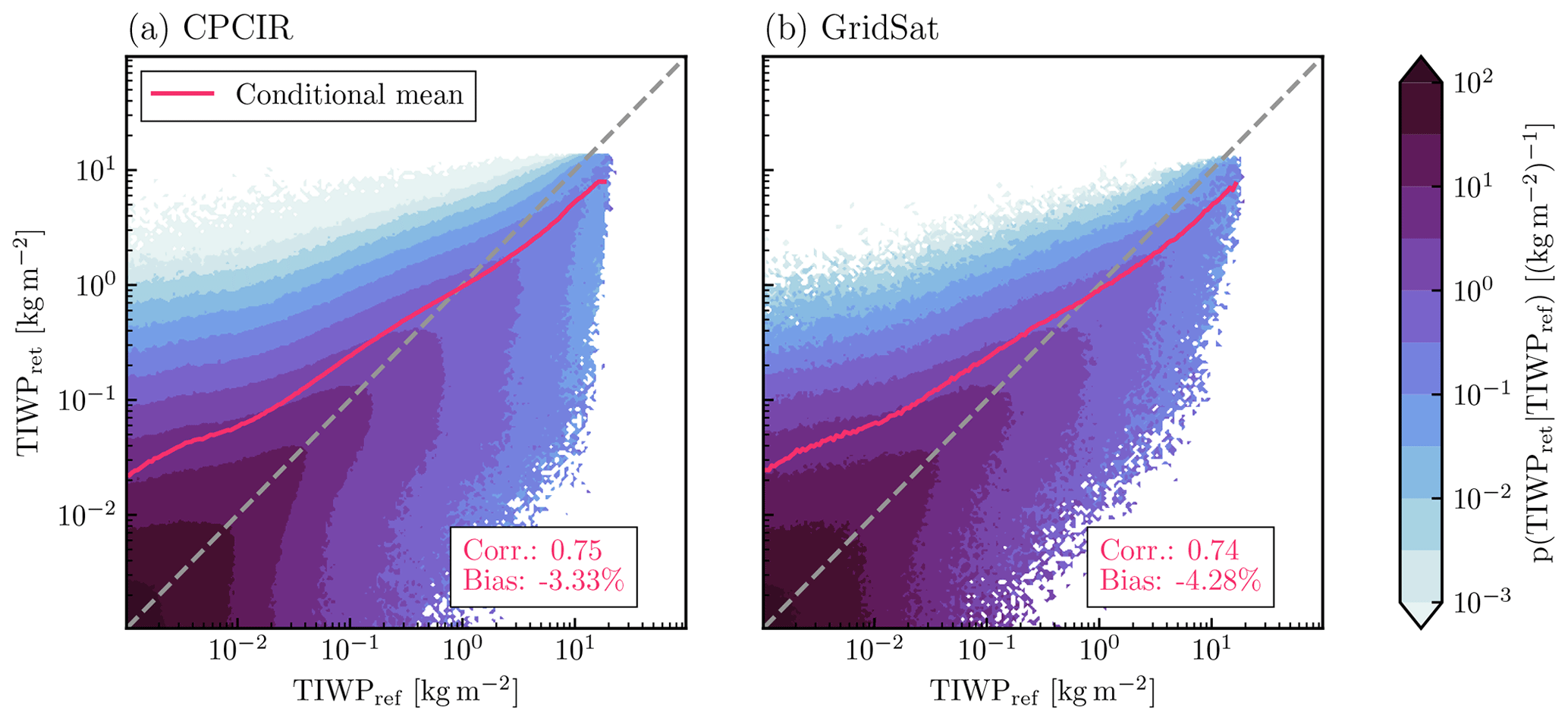
Figure 6 Conditional distributions of retrieved TIWP conditioned on the 2C-ICE-based reference TIWP for the test samples from the year 2010. Panel (a) shows the distribution for the CPCIR input observations; panel (b) shows the corresponding distributions for the GridSat dataset. The displayed bias and correlation coefficients are computed using all test samples including those outside the range of the scatter plot.

In addition to the posterior mean estimate of TIWP, CCIC provides a random sample from the posterior distribution together with a 90 % credible interval (CI). The advantage of random samples from the retrieval posterior distribution is that they provide a better representation of extreme values than estimates relying on the posterior mean. To illustrate this, Fig. 7 shows the zonal distributions of reference and retrieved TIWP values. The retrieval accurately reproduces the zonal variations in the observed TIWP values in terms of both the mean and the distribution of extreme values.

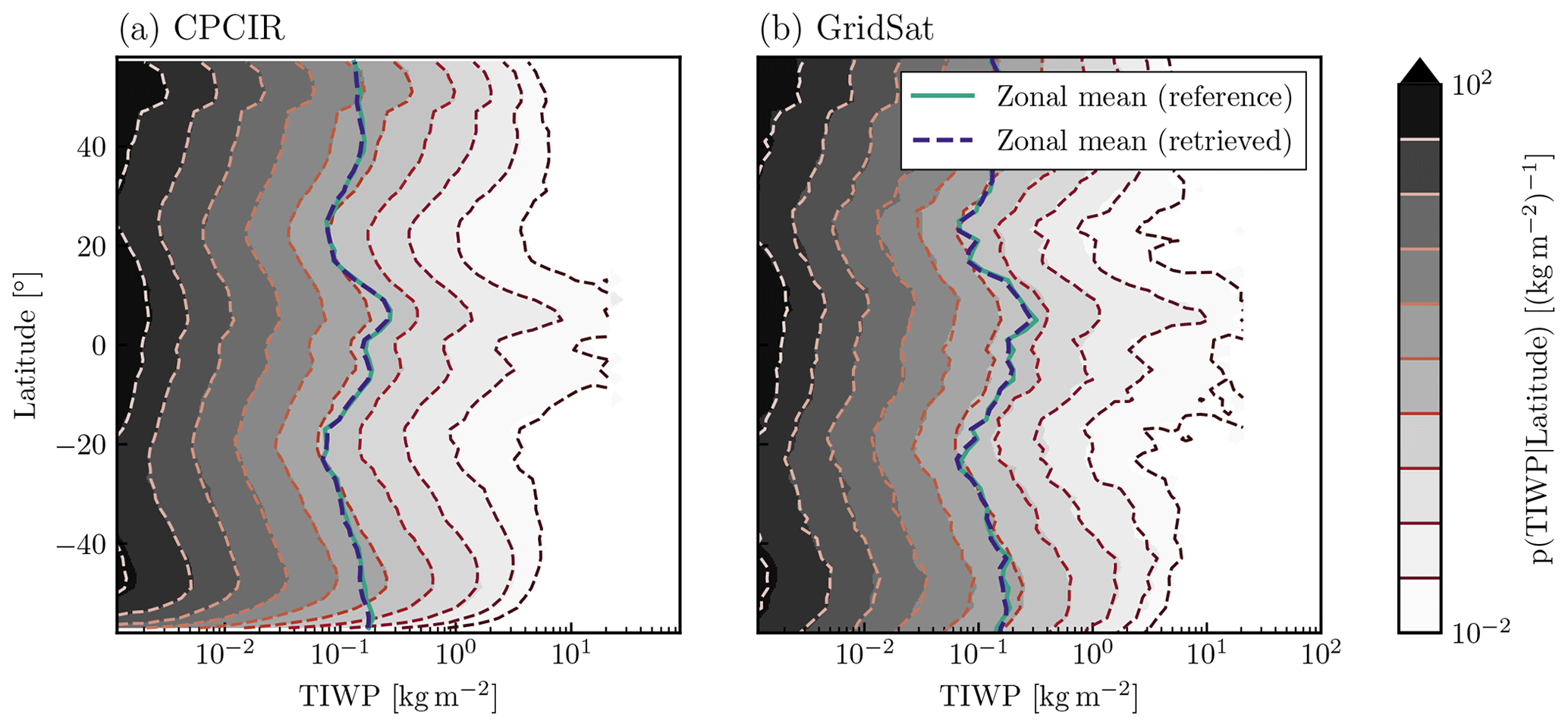
Figure 7 Zonal distributions of retrieved TIWP and 2C-ICE-based reference TIWP for the test dataset. Filled contours in the background shows the conditional probability density function (PDF) of the reference data. Drawn on top are contour lines of the PDF of random samples of the retrieved posterior distribution of TIWP. The contour levels were chosen so that they correspond to the boundaries between the contour levels of the reference data PDF. Line plots show the zonal mean of reference and retrieved TIWP.

The spatial distributions of mean retrieved and reference ice water path (IWP) concentrations from the test dataset are shown in Fig. 8. The distributions of the retrieved TIWP agree well with the distribution of the 2C-ICE measurements. Due to the low number of available 2C-ICE measurements in each 0.5° box, the relative bias field is noisy. The only region where the retrievals exhibit noticeable relative biases is the southeast Pacific dry zone. This is likely caused by the low number of ice clouds in this region in combination with increased relative retrieval uncertainties for low and mixed-phase clouds. Overall, for 90 % of all assessed 5° boxes the biases remain within ±26.54 % (±55.78 %) for the CPCIR-based (GridSat-based) retrievals.

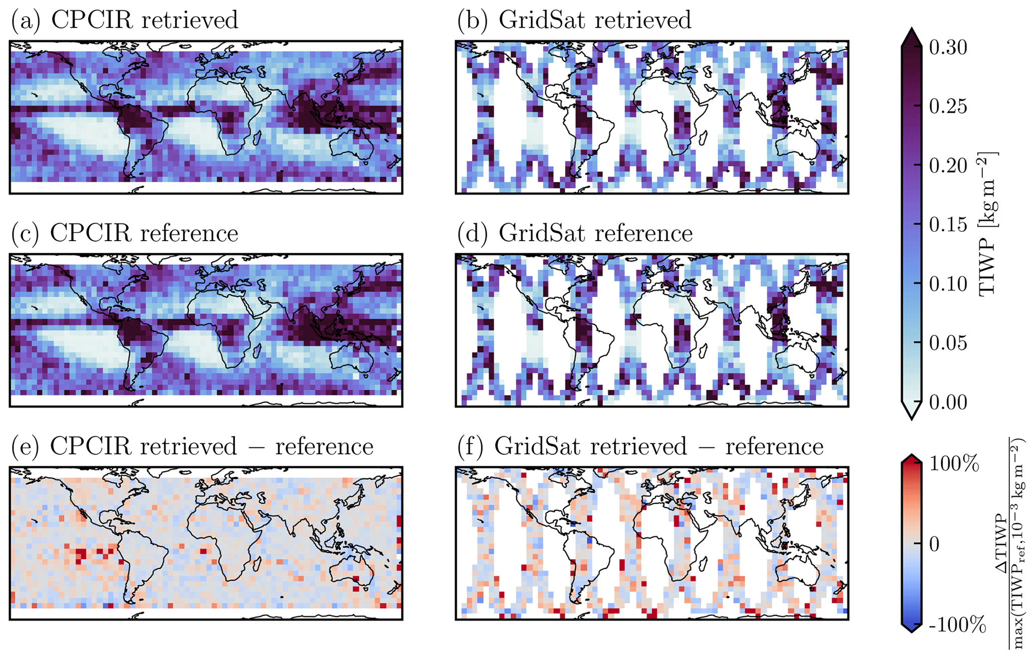
Figure 8 Spatial distribution of retrieved TIWP and 2C-ICE-based reference TIWP for the CPCIR and GridSat test datasets over the domain covered by CCIC. Panels (a) and (b) show the retrieved TIWP aggregated to a resolution of 5°. Panels (c) and (d) show the corresponding distributions of the reference TIWP measurements. Panels (e) and (f) show the relative biases.

Conditional distributions of the retrieved posterior mean TIWC conditioned on reference TIWC at all altitudes are shown in Fig. 9. The distributions exhibit an even larger spread than for the TIWP (Fig. 6), which is expected considering the larger number of degrees of freedom compared to TIWP. Nonetheless, the retrieval achieves low biases and a correlation coefficient exceeding 0.6, thus demonstrating significant skill in reproducing even the vertical distribution of hydrometeors.

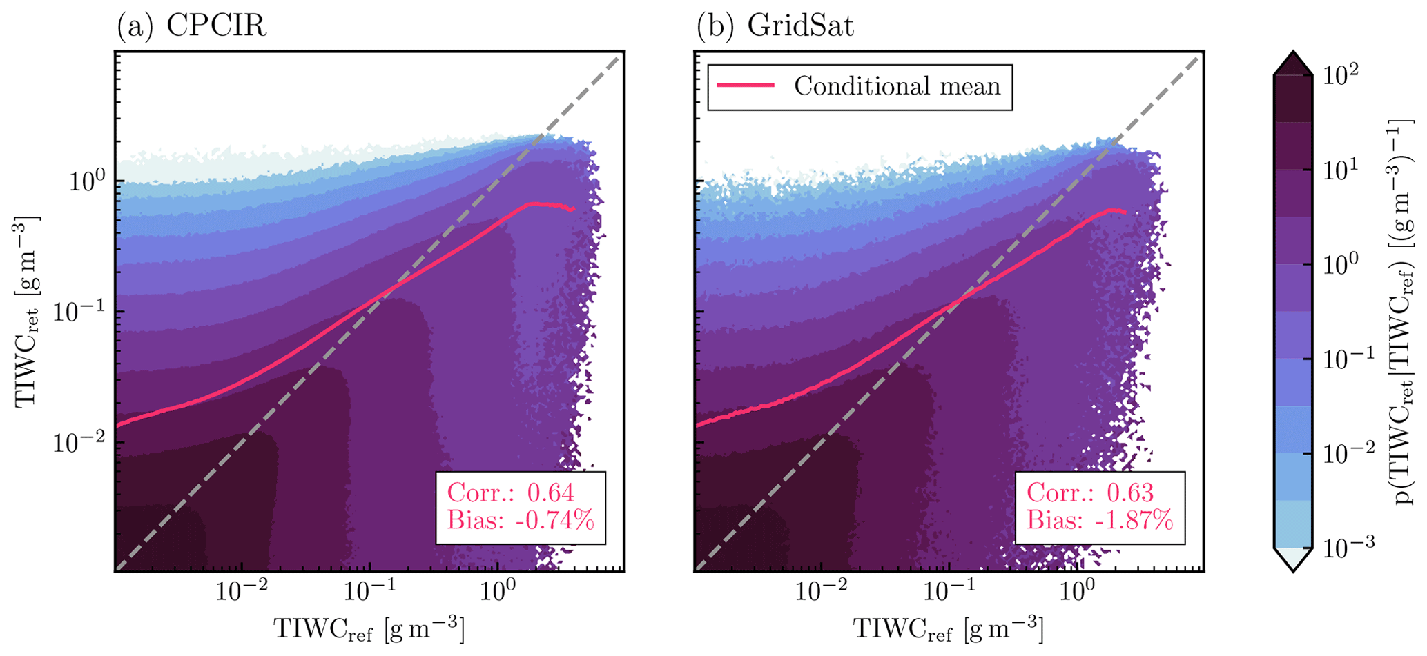
Figure 9 Conditional distributions of retrieved TIWC conditioned on 2C-ICE-based reference TIWC from the test dataset. Panel (a) shows the distribution for the CPCIR input observations; panel (b) shows the corresponding distributions for the GridSat dataset. The displayed bias and correlation coefficients are computed using all test samples including those outside the range of the scatter plot.

Zonal means of all retrieved and reference TIWC estimates are displayed in Fig. 10. Although both retrievals exhibit a tendency to underestimate the TIWC at cloud top and overestimate it at cloud base, the spatial distribution of TIWC is represented well. In particular, the retrievals correctly represent the double-peak structure caused by the seasonal variability in the Intertropical Convergence Zone (ITCZ) as well as the asymmetry of the TIWC distribution in the ITCZ and the storm tracks.

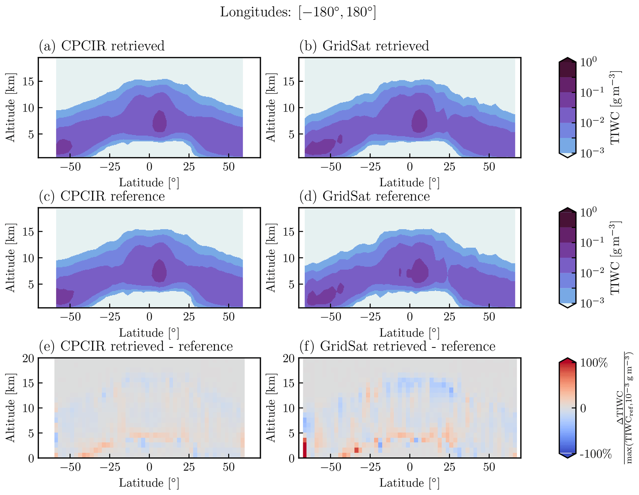
Figure 10 Zonally averaged distributions of retrieved TIWC and 2C-ICE-based reference TIWC for the CPCIR and GridSat test datasets over the domain covered by CCIC. Panels (a) and (c) show the retrieved and reference TIWC for the CPCIR observations aggregated to a resolution of 2.5°. Panel (e) show the truncated relative bias of the retrievals. Panels (b), (d), and (f) show the corresponding distributions of the GridSat-based retrieval.

3.2.2 Consistency of retrieved TIWP and TIWC profiles

Since TIWC is retrieved on evenly spaced altitude levels, the differences in the relative retrieval biases between TIWP (Fig. 6) and TIWC (Fig. 9) indicate small, systematic differences between the retrieved TIWP and the column-integrated retrieved TIWC. When the retrieved TIWP and the column-integrated retrieved TIWC are compared directly, their linear correlation is 1.0 and the overall bias at most 2.52 %. Compared to the reference TIWP, the integrated retrieved TIWC yields slightly smaller biases (−0.72 % and −1.90 % for CPCIR and GridSat, respectively) but similar correlation values. However, since these differences are on the order of a few percent, they can be considered negligible compared to uncertainties in the reference data.

3.2.3 Cloud detection and classification

CCIC provides probabilistic 2D and 3D cloud masks. The 2D cloud mask corresponds to an estimated probability of a cloud being detected by the 2B-CLDCLASS product anywhere in the atmospheric column. The 3D cloud mask classifies all levels in the atmosphere into non-cloudy or any of the eight cloud types distinguished by the CloudSat 2B-CLDCLASS product.

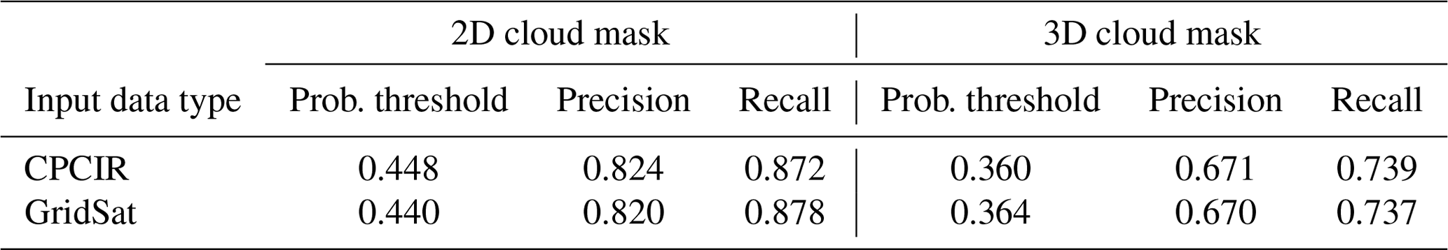
Figure 11 assesses CCIC's skill in detecting clouds in 2D and 3D. The plots display the precision and recall (PR) curves for both input data types. These curves display the trade-off between the precision, i.e., the fraction of correctly identified clouds and the total number of cloud detections, and the recall, i.e., the fraction of correctly identified clouds and the total number of actual clouds, as the probability threshold above which a cloud is counted as detected is varied. The circular markers show the precision and recall for the optimal probability threshold that was determined as the point on the PR curve that is closest (in terms of Euclidean distance) to the point representing a precision and recall of 1. In order to avoid leakage of information from the test data, the optimal decision thresholds were determined using PR curves calculated on the validation data. The corresponding probability thresholds and precision and recall values are listed in Table 4.

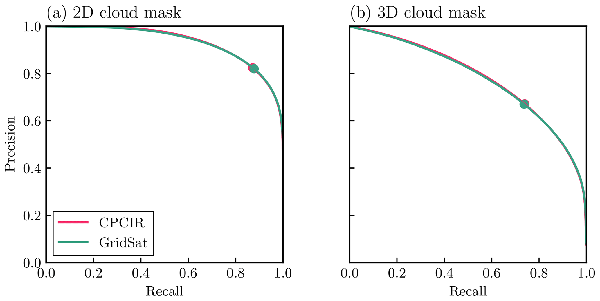
Figure 11 Precision–recall curves for the detection of clouds in 2D and 3D with respect to the 2B-CLDCLASS-based reference data for the test dataset. Panel (a) shows the precision and recall for both input data types for the detection of cloudy columns. Panel (b) shows the corresponding precision and recall for the 3D cloud mask. Circular markers indicate the PR values with the optimal probability threshold in Table 4.

Table 4 Optimal probability thresholds determined with the validation set and corresponding precision and recall for the detection of clouds in 2D and 3D for the test set.

For the detection of clouds in 2D the retrieval achieves a precision and recall in excess of 0.8, indicating good detection skill. For 3D, the detection accuracy decreases, yielding a precision of 0.67 and a recall of around 0.74. Again, the decrease in accuracy for the vertically resolved retrievals is expected due to the higher number of degrees of freedom of the vertically resolved retrieval targets. Nonetheless, these precision and recall values still indicate notable skill in reproducing the horizontal and vertical distribution of clouds in the atmosphere.

The ability of the retrieval to differentiate between the cloud types of the 2B-CLDCLASS product is assessed in Fig. 12, which shows the confusion matrices for each of the two input datasets. The confusion matrix has been normalized to show the conditional probabilities of the retrieved classes given the reference class. High values in the bottom row indicate that all cloud classes have a relatively high chance to be missed. Nonetheless, for all cloud classes except the Cu and the St class, the highest probability is located on the diagonal, indicating the retrieval is able to identify those clouds. However, the retrieval is incapable of distinguishing St from Sc clouds and is more likely to designate an St cloud as Sc than correctly detecting it. The same is true for Cu clouds, which the retrieval is likely to misclassify as Sc, Ns, or DC. It is worth noting, however, that both the St and Sc classes are very rare in the reference data distribution and thus highly unlikely a priori. The imbalanced a priori will lead to biases towards the more likely cloud classes in the conditional distributions.

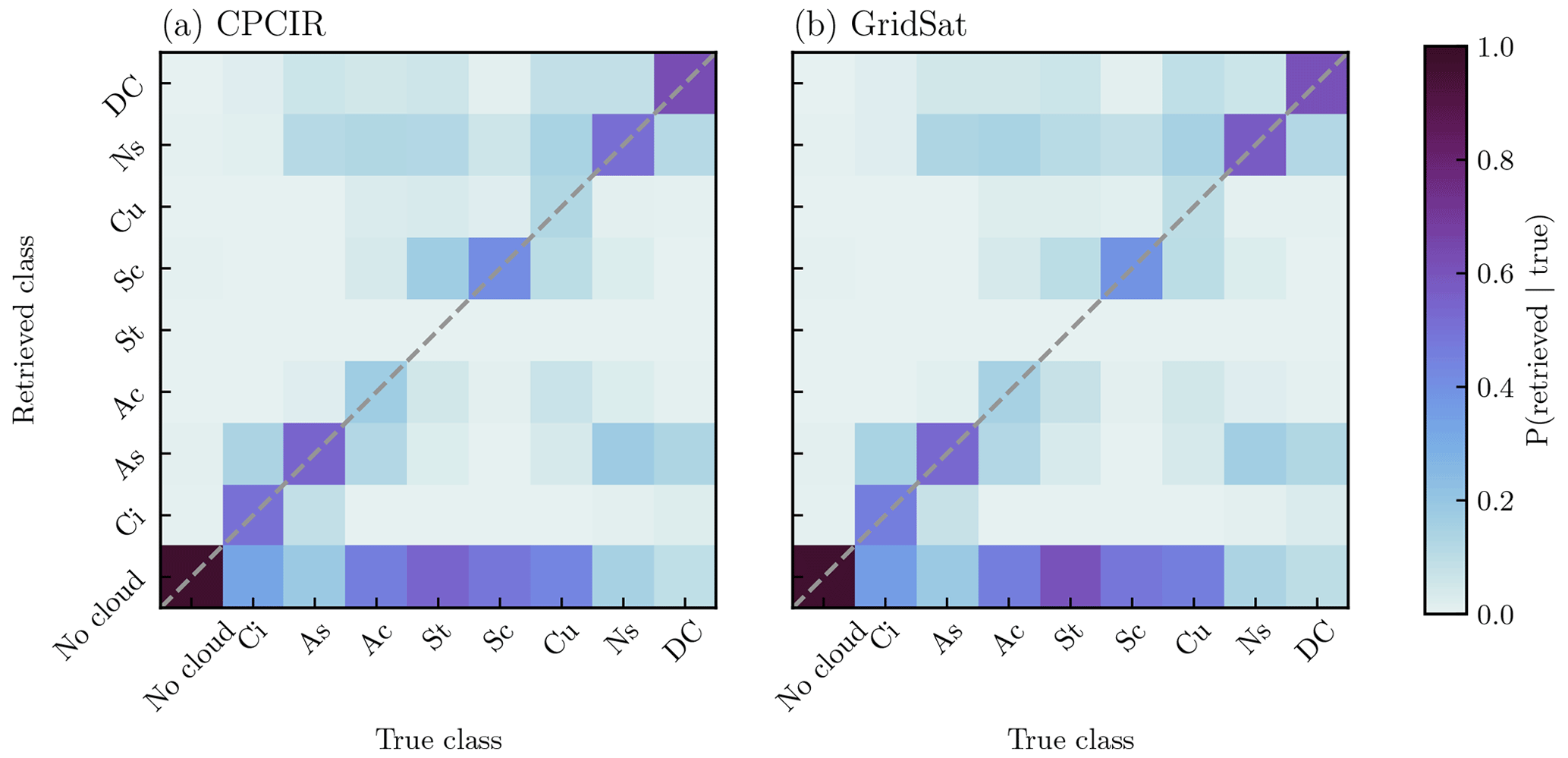
Figure 12 Confusion matrix for the 3D cloud classification. Each matrix shows the conditional probability of the retrieved class given a certain true class. Cloud classes use the acronyms from Table 1.

While the confusion matrix shown in Fig. 12 suggests high uncertainties for the classification of the 1 km vertical levels used by CCIC, the results from the case study shown in Fig. 5 indicate that the retrieval can nonetheless successfully identify the dominant cloud systems in the scene and their vertical extent. To assess the ability of the retrieval to distinguish different cloud systems on larger scales, Fig. 13 shows the frequency of occurrence of the different retrieved and reference cloud types by altitude and latitude band. As these results show, the spatial distribution of the cloud types agrees well with the reference distributions for all cloud types except St, which is never detected. These results confirm that the retrieval has certain skill in distinguishing different cloud systems and their vertical extent despite uncertainties in the classification of individual layers.

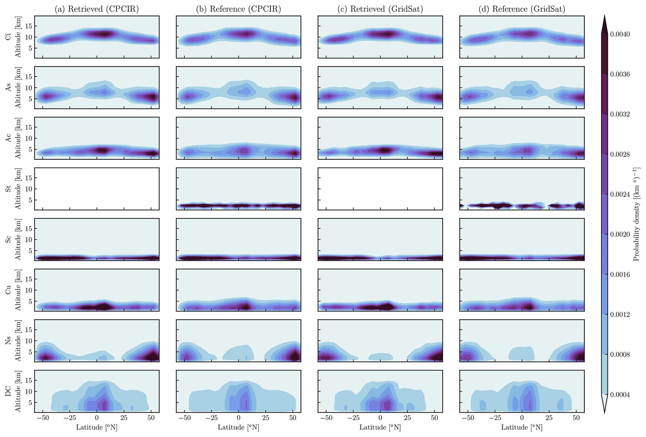
Figure 13 Spatial distribution of retrieved cloud classes and 2B-CLDCLASS-based reference cloud classes for the test samples from the year 2010. Each row of panels shows the distribution of one of the eight cloud classes distinguished by the 2B-CLDCLASS product. The first column shows the results retrieved from CPCIR observations, while the second column shows the corresponding reference distribution. Columns three and four show the corresponding results for retrievals based on GridSat observations.

4 Validation

The evaluation of the retrieval accuracy on the test data presented in the previous section showed that the CCIC retrieval is able to reproduce the CloudSat reference measurements well. However, the scientifically more relevant question is whether the retrieval can provide reliable estimates even in comparison to independent measurements. If CCIC can reliably characterize distributions of frozen hydrometeors even outside the temporally and spatially limited sampling of the CloudSat reference measurements, CCIC would be able complement the CloudSat data record by providing spatially and temporally continuous measurements around much of the globe, albeit at reduced resolution and accuracy. To investigate this question, this section compares CCIC retrievals to measurements of cloud hydrometeors from several flight campaigns and ground-based cloud radar measurements.

4.1 HAIC-HIWC

4.1.1 Case study

A case study comparing airborne radar and in situ measurements from the Darwin campaign of the HAIC-HIWC project and CCIC retrievals is shown in Fig. 14. The flight probed the anvil and core of a deep convective system in the Gulf of Carpentaria. In the beginning of the flight, the aircraft passed through low-level clouds while still close to Darwin. The aircraft entered the anvil of the system at around 21:00 UTC and then passed through the core of the system several times. Overall, both CCIC retrievals capture the horizontal and vertical extent of the observed cloud fairly well. However, the CPCIR-based retrieval overestimates the horizontal extent of the anvil cloud. A potential explanation for this is that during the time of the campaign, the CPCIR input data around Darwin are missing at the full hour, and the results at 21:00 UTC are thus linearly interpolated between the results at 20:30 and 21:30 UTC. In contrast to that, the GridSat-based retrieval, which has valid input observations at 21:00 UTC, reproduces the horizontal extent of the anvil cloud more accurately.

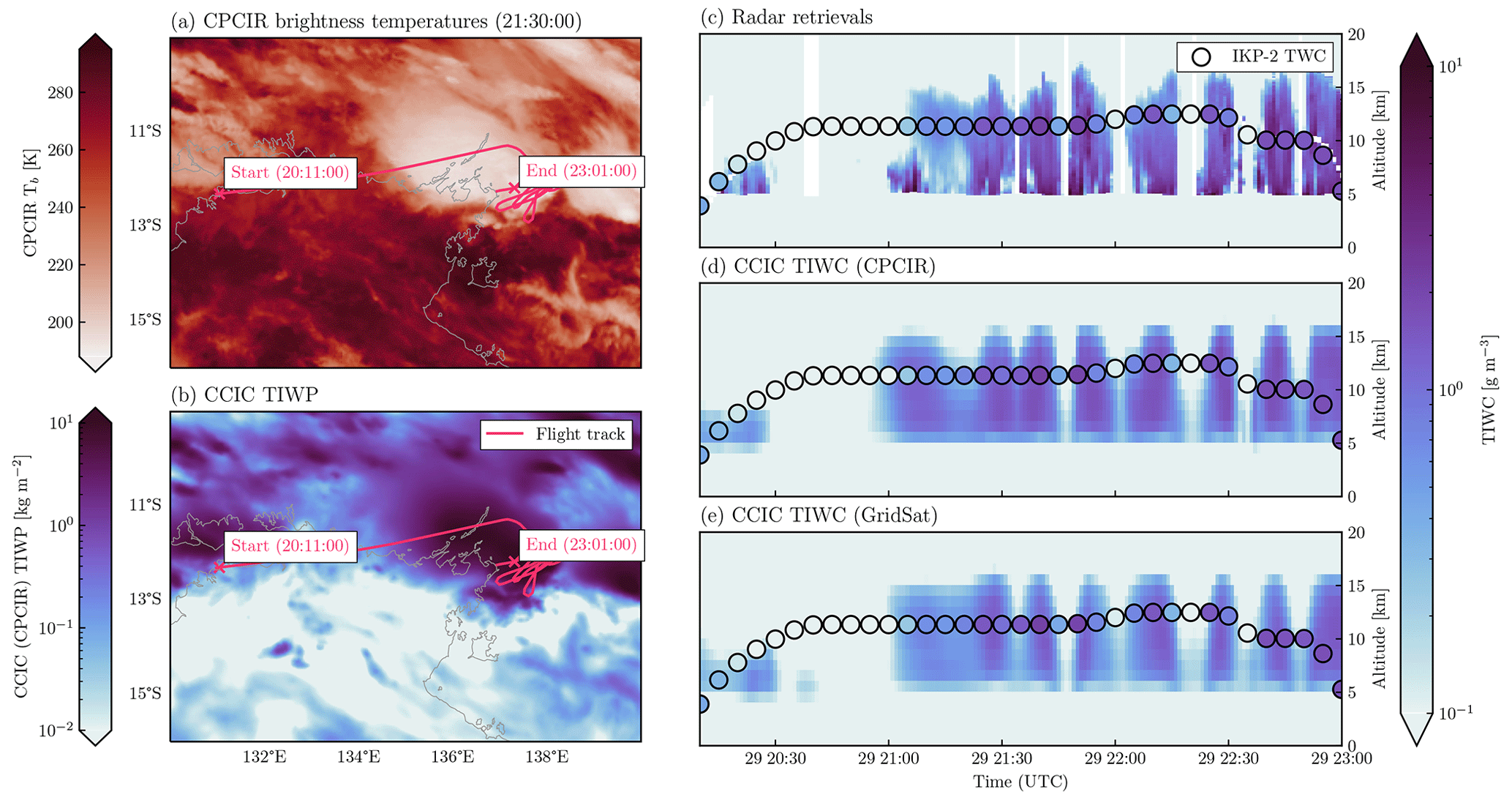
Figure 14 In situ measurements and retrieval results for flight 10 of the Darwin HAIC-HIWC campaign on 29 January 2014. Panel (a) shows the CPCIR 11 µm brightness temperatures. Panel (b) shows the corresponding CCIC TIWP field. Panel (c) shows the TIWC retrieved from the RASTA cloud radar using the large-column aggregate as ice particle shape. Circular markers show the 5 min average TWC measured in situ from the IKP-2 probe. Panels (d) and (e) show the TIWC retrieved from CPCIR and Gridsat observations and interpolated to the flight path.

The CCIC retrievals are not able to capture the internal structure of the clouds and slightly underestimate the variability in the magnitude of the TIWC between the anvil and the core of the convective system. To a certain extent this is expected considering the very limited information provided by the single-channel IR observations used as input from the retrieval. Nonetheless, it is notable that the CCIC retrieval, at least to first order, yields estimates of TIWC that are consistent with both the radar and the in situ measurements.

4.1.2 HAIC-HIWC: aggregated data

For a broader comparison of the CCIC retrievals and the campaign measurements, Fig. 15 shows the distributions of retrieved TIWC conditioned on in situ measurements from all HAIC-HIWC campaigns. The CCIC retrievals exhibit a tendency to overestimate TIWC at concentrations below 0.1 g m⁻³ and underestimate it above 1 g m⁻³. Overall, however, the CCIC-retrieved TIWC is reasonably well correlated with the HAIC-HIWC in situ measurements across all campaigns of the project.

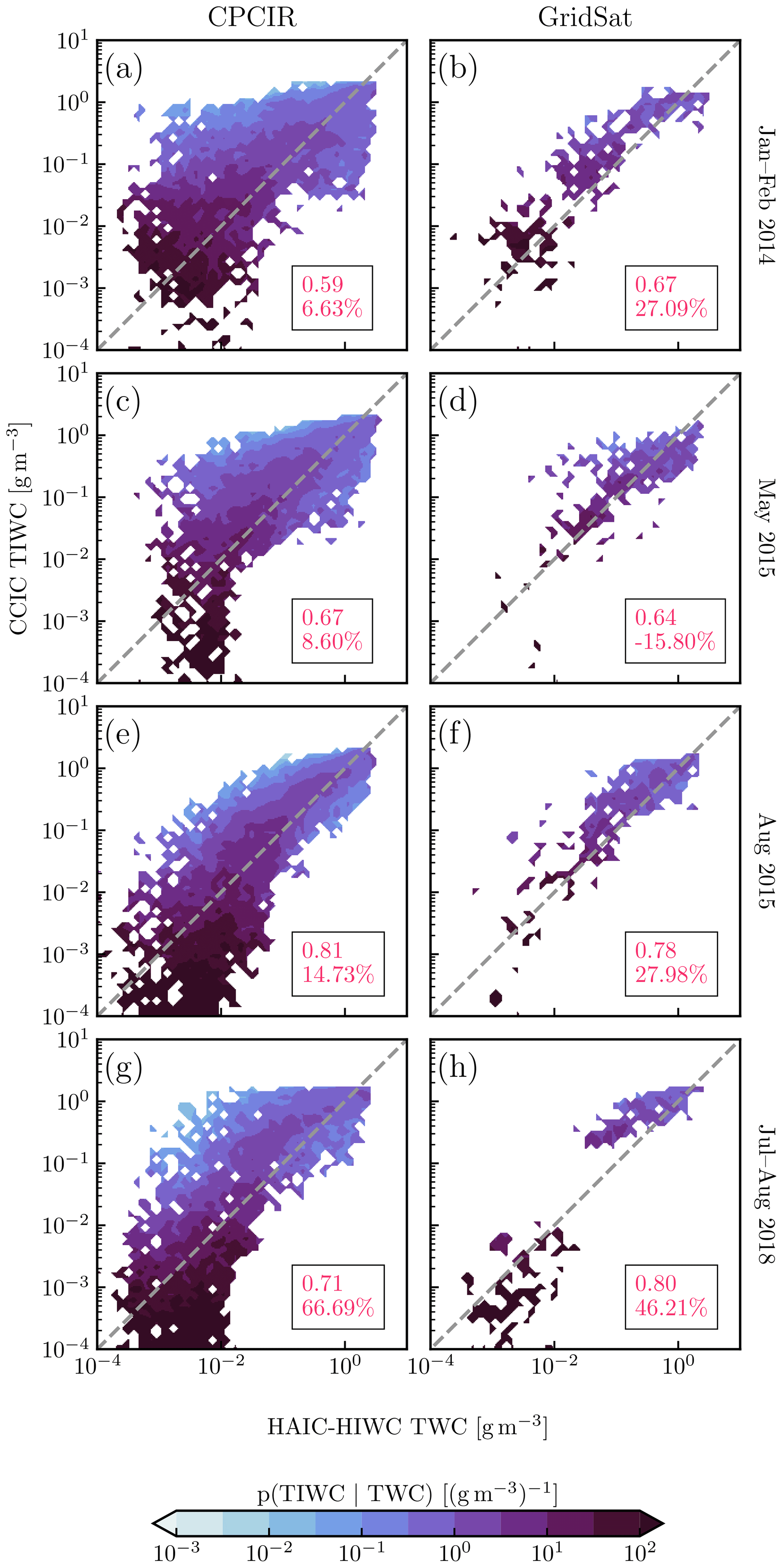
Figure 15 Distributions of retrieved TIWC conditioned on reference TIWC from the in situ measurements for each of the HAIC-HIWC campaigns presented in Fig. 3. The left column contains CPCIR retrievals and the right column GridSat retrievals; the first number in the box indicates the correlation and the second the bias. The displayed bias and correlation coefficients are computed using all test samples including those outside the range of the scatter plot.

Scatter plots of CCIC-retrieved TIWC and TIWP conditioned on reference retrievals from the RASTA airborne cloud radar used during the Darwin campaign are shown in Fig. 16. The radar retrievals for the HAIC-HIWC campaign use the large-column aggregate particle model, which yielded the best agreement with collocated in situ measurements (see Appendix C). With respect to TIWC, the overestimation and underestimation tendencies are consistent with the validation against the in situ measurements, and the retrieved values also are reasonably well correlated against the reference values. In terms of TIWP, the CCIC retrievals are biased high for reference values below 1 kg m⁻², but the overall bias remains comparably low. With values of 0.66 and 0.62 for the CPCIR and GridSat-based retrievals, respectively, the correlations are higher than for the TIWC estimates.

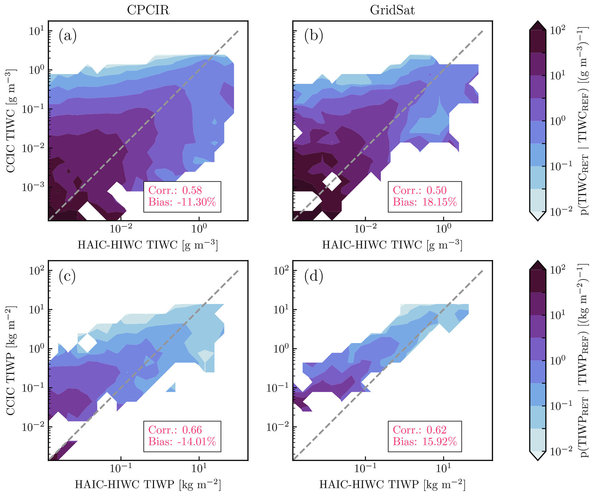
Figure 16 Distributions of retrieved TIWC (a, b) and TIWP (c, d) conditioned on reference values from airborne radar retrievals during the Darwin HAIC-HIWC campaign (January–February 2014) obtained with the large-column aggregate particle model. The displayed bias and correlation coefficients are computed using all test samples including those outside the range of the scatter plots.

4.2 OLYMPEX

A case study depicting CCIC retrieval results together with in situ measurements and TIWC derived from radar observations from the NASA CRS is shown in Fig. 17. The depicted flight is the one that allowed for the largest number of collocations between radar retrievals from the NASA CRS system on the ER-2 aircraft and the in situ probes on the UND Citation aircraft. During the flight the two aircraft profiled a prefrontal storm over the Olympic Peninsula. The radar retrievals show the vertical extent of cloud extending up to 8 km and decreasing down to 3 km towards the end of the flight leg. The CCIC retrievals from the CPCIR observations capture the overall shape of the cloud system but overestimate its vertical extent. The GridSat-based retrieval is even less successful in reproducing the extent of the cloud. This is likely due to the lower temporal resolution of the input data, which required interpolation between the available results at 15:00 and 18:00 UTC.

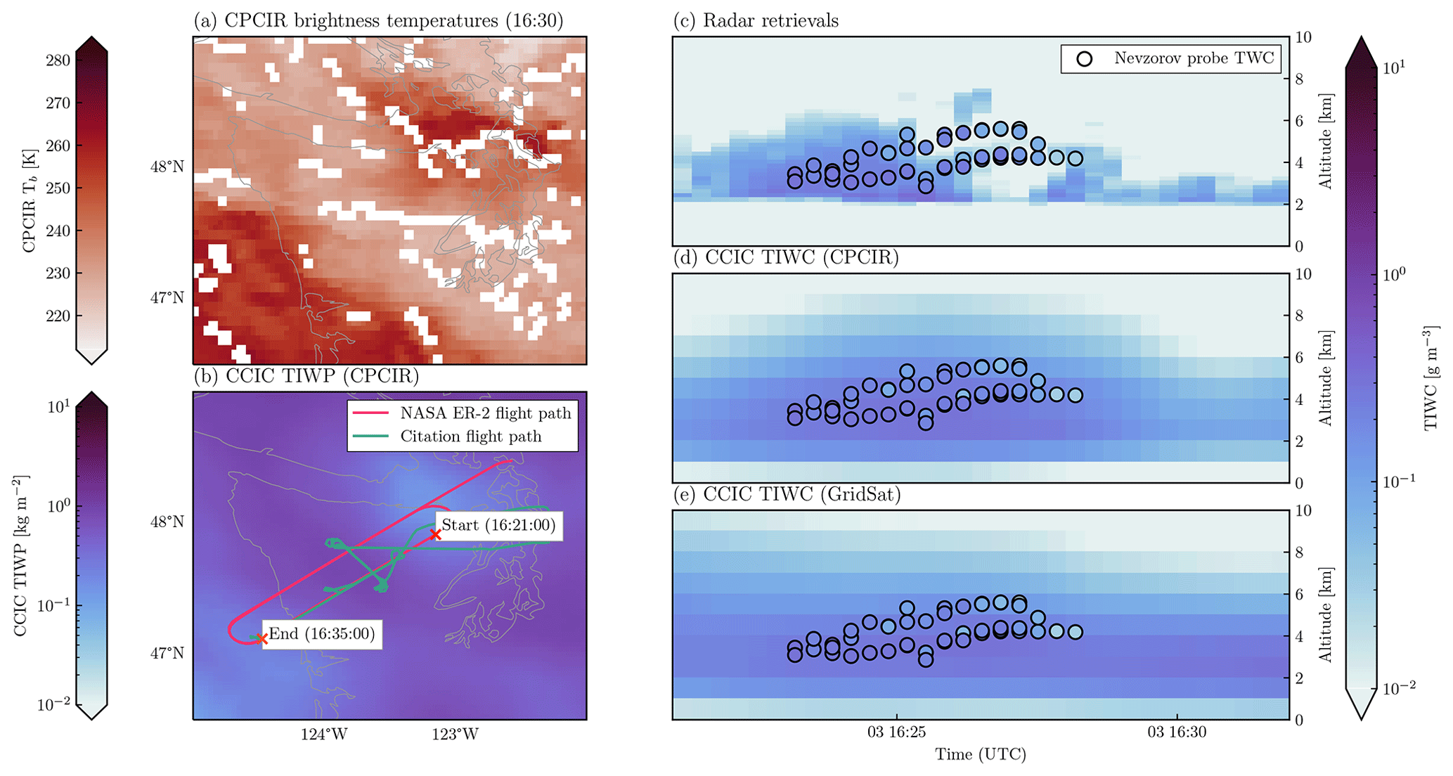
Figure 17 Collocated in situ, radar, and CCIC measurements of ice hydrometeors from a flight on 4 December 2015 during the OLYMPEX campaign. Panel (a) shows the CPCIR input data for the CCIC retrieval over the Olympic Peninsula. White pixels mark missing values in the input data. Panel (b) shows the corresponding retrieved TIWP. Panel (c) shows the TIWC retrieved from the NASA CRS on the ER-2 aircraft using the large-plate aggregate ice particle model. Scatter points show collocated Nevzorov probe measurements of TWC from the UND Citation aircraft within 5 km and 15 min of the radar observations. Panel (d) shows TIWC along the flight path derived from CPCIR input data. Panel (e) shows the TIWC derived from GridSat observations.

The radar observed broken clouds from about 16:25 to 16:28 UTC, while the in situ measurements exhibit spatially more continuous hydrometeor concentrations. The broken clouds observed by the radar indicate high spatial and temporal variability in the cloud field that is too high for the CCIC retrievals to resolve, thus leading to the overestimation of the vertical extent of the cloud system. It should also be noted that the in situ measurements indicate the presence hydrometeors even where no cloud is observed in the radar measurements, providing further evidence that deviation between radar, in situ, and CCIC measurements is, at least in part, due to the variability in the cloud field.

Scatter plots of the conditional distribution of retrieved TIWC conditioned on reference TWC and TIWC are displayed in Fig. 18. Compared to the in situ measurements, the CPCIR CCIC results are biased high and exhibit relatively low correlation of 0.36. With a value 0.65, the correlations are significantly higher for the GridSat retrievals. Since all other comparisons showed a high degree of similarity between the CPCIR and GridSat-based results, the higher correlation is probably due to the spatial and temporal sampling of the collocations used for the validation of the GridSat-based results. The GridSat-based retrievals also exhibit a weaker bias in the TIWC estimates. The correlations with respect to the airborne radar measurements are significantly higher with values of 0.6 for the CPCIR-based retrievals and 0.73 for the GridSat-based retrievals. The biases with respect to the radar measurements are similar to those observed for the in situ measurements. The radar results shown here were obtained with the large-plate aggregate particle model. Although the few available collocations between radar and in situ measurements showed the best agreement for the eight-column aggregate particle model, the large-plate aggregate led to better agreement between the biases between radar estimate and CCIC and in situ measurements and CCIC.

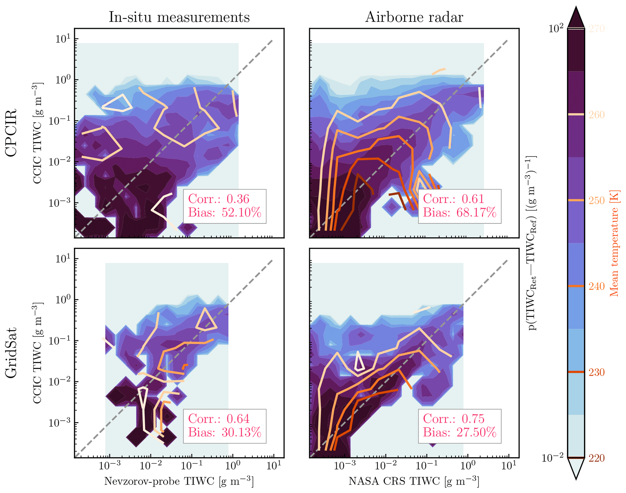
Figure 18 Distributions of retrieved TIWC conditioned on reference TIWC measurements during the OLYMPEX campaign. Contour lines show the mean of the ERA5-derived ambient temperature for the retrieval results in each bin. The displayed bias and correlation coefficients are computed using all test samples including those outside the range of the scatter plots.

The conditional distributions show that the CCIC retrievals severely overestimate TIWC for low reference concentrations in some cases. The temperature contours indicate that these cases of overestimation are associated with comparably high temperatures and thus correspond to estimates lower down in the atmosphere, where the input observations provide little information to guide the retrieval. Moreover, the limited vertical resolution and lack of input data constraining the thermal structure of the atmosphere may lead to TIWC being retrieved close to and even below the freezing level.

Finally, scatter plots showing the distributions of retrieved TIWP conditioned on the radar-retrieved TIWP are shown in Fig. 19. Although the spread in the distributions TIWP is reduced compared to the radar-measured TIWC, the correlation with the reference measurements decreases for the CPCIR retrievals. The reduction in correlation for the TIWP retrievals is somewhat surprising considering that TIWP should be easier to retrieve due to the lower number of associated degrees of freedom. What may contribute to the reduced correlation, however, is the relatively low sensitivity of the radar retrievals, which is evident in the lack of reference measurements of TIWP values below 10⁻² kg m².

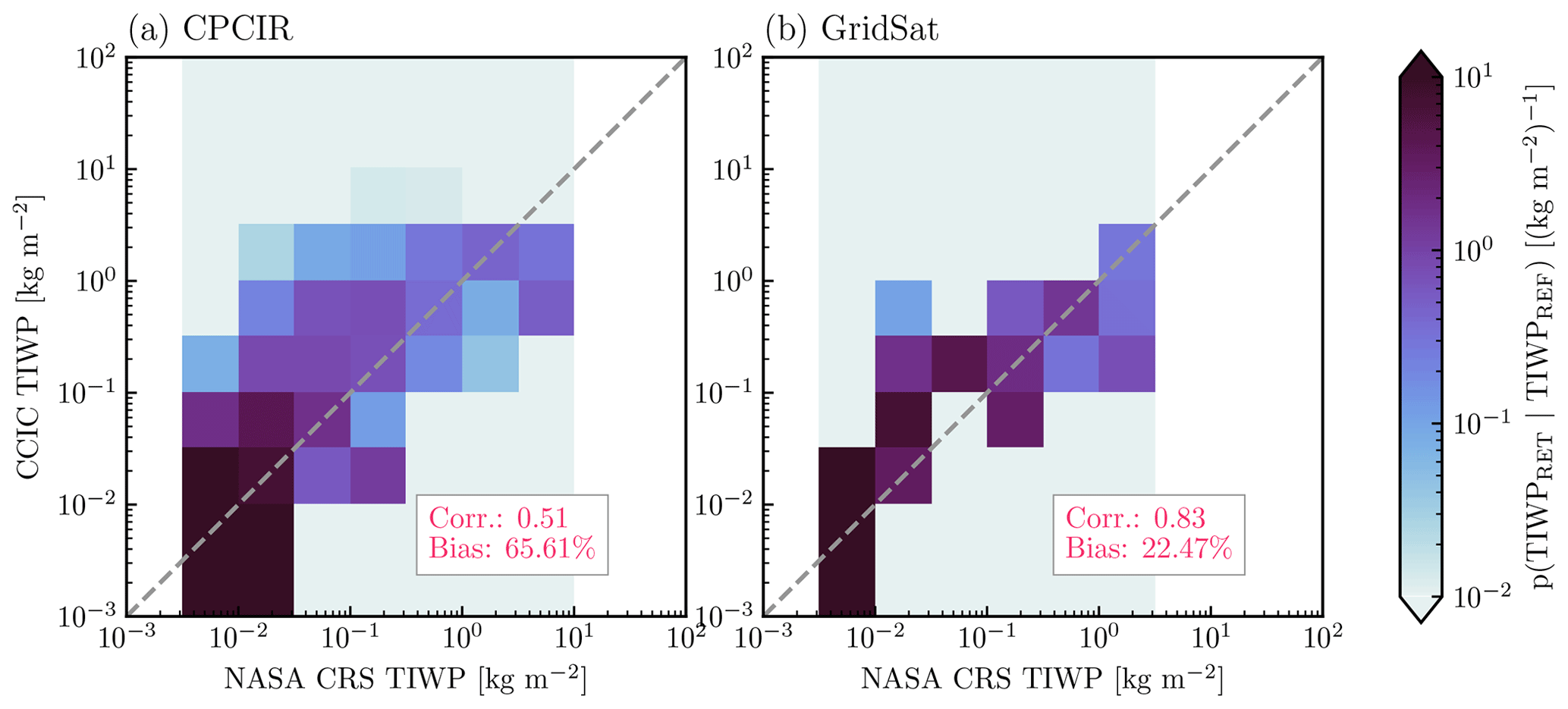
Figure 19 Distributions of retrieved TIWP conditioned on cloud-radar-derived reference TIWP measurements during the OLYMPEX campaign. The displayed bias and correlation coefficients are computed using all test samples including those outside the range of the scatter plots.

4.3 Cloudnet

Figure 20 compares CCIC retrievals with TIWC and TIWP estimates derived from the Cloudnet ground-based cloud radar in Palaiseau. The conditional distributions of collocated TIWP and TIWC exhibit a similar spread to the flight campaigns but with slightly lower correlations. The CCIC retrievals overestimate hydrometeor concentrations by 30 % to 40 % compared to radar retrievals using the large-plate aggregate particle model.

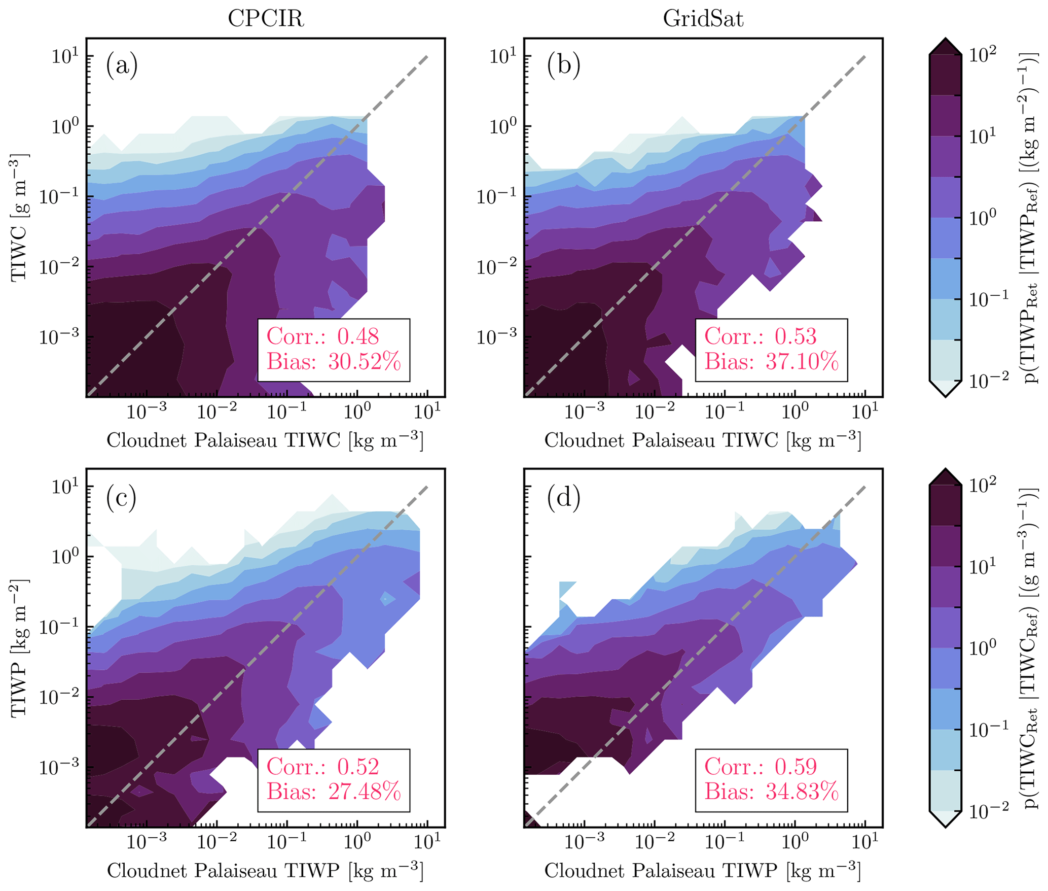
Figure 20 Conditional distributions of retrieved TIWP (a, c) and TIWC (b, d) retrievals conditioned on reference measurements from the ground-based cloud radar in Palaiseau. The first row shows the results for the CPCIR-based CCIC retrievals. The second row shows the results for the GridSat-based CCIC retrieval. The displayed bias and correlation coefficients are computed using all test samples including those outside the range of the scatter plots.

Figure 21 shows diurnal cycles of TIWP retrieved from the ground-based radar and the CCIC retrievals. Calculated over the full year 2019, the CCIC retrievals reproduce the TIWP peak in the morning but underestimate the reduction in TIWP occurring around 15 h. The CCIC retrievals capture most of the seasonal variation in the diurnal cycle. The exception is the summer months, during which the CCIC results capture the general shape of the diurnal cycle but underestimate the magnitude of the variation. Nonetheless, as shown in Table 5, the correlation of the retrieved diurnal cycles and those derived from radar simulations using the large-plate aggregate particle model exceeds 0.7 during all seasons. Due to their lower temporal resolution, the GridSat-based results generally exhibit weaker variations than the CPCIR retrievals but yield higher correlations compared to the reference diurnal cycles calculated at 3h resolution.

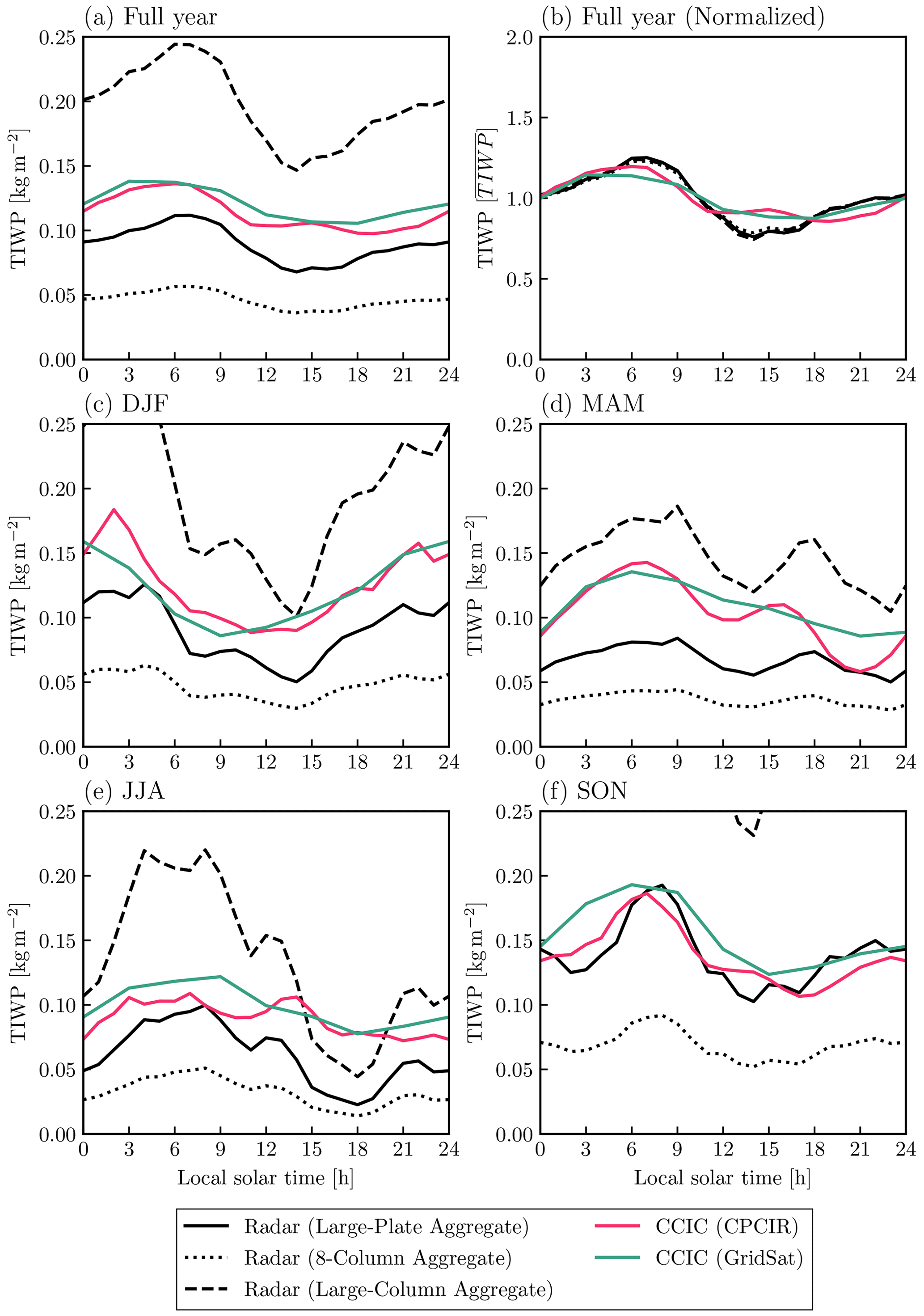
Figure 21 Diurnal cycles of TIWP retrieved from CCIC and the Cloudnet ground-based cloud radar in Palaiseau. Panel (a) shows the diurnal cycles in absolute TIWP values. Black lines show the retrieved diurnal cycles for the three different particle models used in the radar retrievals. Panel (b) shows diurnal cycles normalized by the mean TIWP. Panels (c)–(f) show seasonal diurnal cycles.

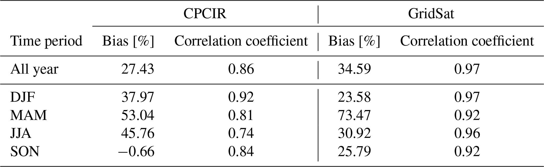
Overall, it is notable that the CCIC retrievals manage to reproduce the diurnal and seasonal variation relatively well, as presented in Table 5: the linear correlation between retrievals from CCIC and the Cloudnet radar used is at least 0.74 for any of the assessed 3-month periods. It is important to note that CloudSat measurements are essentially limited to two discrete local overpass times due to the sun-synchronous orbit of the satellite. Therefore, they cannot resolve the diurnal cycle of cloud properties. The good agreement with the ground-based measurements shows that, despite being based on CloudSat measurements, the CCIC retrieval can reproduce diurnal variations in TIWP. The CCIC retrievals thus have the potential to provide an important novel perspective on ice clouds in the atmosphere.

Table 5 Relative bias and linear correlation coefficient of the diurnal cycles retrieved using CCIC compared to those derived from the Cloudnet ground-based cloud radar in Palaiseau using the large-plate aggregate particle model.

5 Discussion

This study introduced the CCIC ice cloud retrieval that produces estimates of TIWP, TIWC, and cloud coverage from single-channel geostationary IR observations. The input data were deliberately restricted to a single channel of geostationary observations so that the retrieval could be applied to the entire historical record of geostationary satellite observations. To demonstrate the soundness of the concept and its implementation, we have presented a thorough assessment and validation of the neural-network-based retrieval.

5.1 Retrieval accuracy

The assessment of the retrieval accuracy on the held-out test dataset (Sect. 3) showed that the CCIC retrieval can reliably reproduce the CloudSat 2C-ICE estimates, although individual retrievals may exhibit considerable uncertainty. CCIC can even reproduce the vertical distribution of ice hydrometeors despite its input being limited to a single channel of IR observations. This is certainly notable, especially since it is commonly understood in the remote sensing community that broader spectral coverage is required to reproduce the vertical structure of clouds.

This study further validated the retrieval against measurements from two flight campaign series and a ground-based cloud radar. The CCIC retrievals generally agree with the radar measurements and most in situ measurements. The biases with respect to in situ measurements were within or close to 50 % for both flight campaign series, which is an encouraging result considering that biases in combined radar–lidar retrievals, which are taken as reference estimates here, can be up to 59 % for comparisons against in situ measurements (Deng et al., 2013a). The lowest sensitivity was found for the CPCIR-based retrievals for the OLYMPEX campaign where the correlation with the in situ measurements was only 0.36. The likely reason for this is that the in situ measurements from the UND Citation aircraft mostly sampled altitudes close to the cloud base where the retrieval uncertainties are highest. This is confirmed by the much better correlation coefficient found for the comparison to the radar-derived TIWC measurements. The otherwise good agreement between in situ measurements and CCIC TIWC retrievals confirms the ability of the retrieval to resolve the vertical distribution of ice hydrometeors in the atmosphere.

The validation data covered the time range 2014–2020 and climatic regimes from the tropics to the midlatitudes. The fact that the CCIC retrieval yields reliable results even far outside of the period used for training the retrieval (2006–2009) constitutes preliminary evidence that the retrieval results are stable in time. Moreover, CCIC exhibits comparable sensitivity (measured in terms of correlation with the campaign measurements) and biases for both tropical and midlatitude cloud regimes, indicating robustness of the retrieval across climate zones. In general, the CCIC retrievals tend to overestimate in situ and radar measurements. This is consistent with a similar tendency to overestimate hydrometeor concentrations measured in situ found for the 2C-ICE product (Deng et al., 2010, 2013b), which is used as reference data to train the CCIC retrieval.

Overall, the validation results are very encouraging and indicate that CCIC provides reliable results that constrain not only the integrated density of frozen hydrometeors but also their vertical distribution. Moreover, good agreement with the diurnal cycles derived from the ground-based radar shows that CCIC complements currently available A-Train-based measurements by providing retrievals outside their limited spatial and temporal coverage.

CCIC's objective is to improve the observational climate record of ice hydrometeor concentrations using modern deep-learning techniques. We aim to produce a full climate record of cloud retrievals but acknowledge that the long-term stability of these deep-learning-based retrievals remains an open question, which we aim to address in a follow-up study. Because of the exploratory character of CCIC (and the limited funding available for the project), there is likely room to improve the retrieval further. Although based on the state-of-the-art ConvNeXt architecture, the employed neural network architecture has yet to be optimized exhaustively. Further potential opportunities for improving the retrieval are unsupervised pre-training and incorporating the temporal evolution into the retrieval.

5.2 Limitations

Since CCIC uses the 2C-ICE and 2B-CLDCLASS products as reference data, it will directly inherit their characteristics. In particular this means that CCIC is based on the same microphysical assumptions as these two products and will therefore reproduce their errors. The 2C-ICE product uses a modified gamma particle size distribution (PSD) with a habit mixture of randomly oriented particles to retrieve TIWC from combined CloudSat and CALIPSO measurements (Deng et al., 2010); however, since it does not provide detailed information regarding the properties of the particles, it is not possible for us to assess the impact of those assumption. Nonetheless, our validation showed that the resulting CCIC estimates agree reasonably well with in situ measurements, thus instilling confidence in the reliability of both the reference data and the CCIC retrievals.

A principal difficulty of measuring concentrations of hydrometeors in the atmosphere is establishing a ground truth. In situ measurements are difficult to conduct and are therefore rare. Furthermore, available measurements have to be collocated with satellite-based retrievals, whose measurements typically extend over significantly larger measurement volumes. Since both flight campaigns considered here comprised a relatively large number of flight hours, we were able to average the campaign measurements to the native resolution of the satellite retrievals. While this yielded fairly good agreement, we note that, despite the averaging, the measurement volumes are likely to remain vastly different, which will contribute to the error between retrieval and validation data.

Quantitative estimates of hydrometeor concentrations derived from radar measurements exhibit significant uncertainty due to their sensitivity to the assumed microphysical properties, which are difficult to constrain a priori. The approach taken here was to perform multiple radar retrievals with different assumptions on the particle shape and constrain the results through comparison with the in situ measurements. This worked well for the HAIC-HIWC campaign, for which the best agreement between radar and in situ measurements was found for the large-column aggregate particle model, but led to inconsistencies in the biases between CCIC and the OLYMPEX campaign in situ measurements and radar retrievals. For OLYMPEX we therefore chose the large-plate aggregate as the most suitable particle model and used the same for the Palaiseau results, where it led to fairly good agreement between radar and CCIC retrievals. While the results are reasonably consistent, we note that microphysical assumptions constitute a major uncertainty for the radar retrievals used in this study.

Since CCIC was designed to be applied to geostationary observations, its retrievals are currently limited to the range −60° N (−70° N) to 60° N (70° N) for the CPCIR-based (GridSat-based) retrievals. We are confident that the approach could also be applied to high-latitude and polar regions using observations from polar-orbiting satellites such as those used by the PATMOS-x dataset. While cloud retrievals of low clouds over snow-covered surfaces present specific technical difficulties, the machine-learning-based approach could benefit from improved spectral information provided by advanced very high-resolution radiometer (AVHRR)-type sensors and the increased coverage of CloudSat–CALIPSO observations in high-latitude and polar regions.

5.3 Applications

Given that CCIC uses only single-channel IR observations as retrieval input, an important question to answer is whether CCIC's retrievals add new information that cannot be readily obtained from the input data. To address this question, the following subsections discuss two possible applications where the CCIC retrievals may provide an advantage over the original IR brightness temperatures.

5.3.1 Cloud tracking

A common application of IR observations from geostationary satellites is the tracking of convective cloud systems. Tracking algorithms typically use IR brightness temperatures to identify cold clouds (Feng et al., 2021; Esmaili et al., 2016; Fiolleau and Roca, 2013). The issue with this is that IR brightness temperatures reflect the location of the cloud top with respect to the thermal structure of the atmosphere rather than the processes forming the cloud. Since the CCIC retrievals can reproduce the vertical structure of clouds and identify different cloud types, the CCIC results may provide a better way to identify and track cloud systems. While the most natural way of tracking cloud systems would be using the cloud detection outputs provided by CCIC, this approach has the disadvantage of not having a direct correspondence in the output fields from climate models, which is often desired to allow comparison of model- and observation-derived tracking databases. However, it seems reasonable to assume that also the TIWP field provides a more direct signal to track clouds than the IR brightness temperatures.

The global mesoscale convective system database by Feng et al. (2021), for example, uses a threshold of 225 K to identify a deep convective core and tracks the surrounding cold cloud shield consisting of surrounding pixels with brightness temperatures below 241 K. The ability of the raw IR brightness temperatures and the CCIC-retrieved TIWP fields to identify convective clouds and associated cloud shields can be assessed with the test data used in Sect. 3. To this end, we classify an atmospheric column associated with a pixel of CPCIR observations as cloudy and convective based on the corresponding cloud scenario from the 2B-CLDCLASS product. A pixel is classified as cloudy if the corresponding column contains a cloud at least at one level. Similarly, it is classified as convective if it contains a Cu, Nb, or deep convective cloud anywhere in the column. Figure 22 shows precision–recall curves for the detection of clouds and the detection of convective pixels using different brightness temperature and TIWP thresholds.

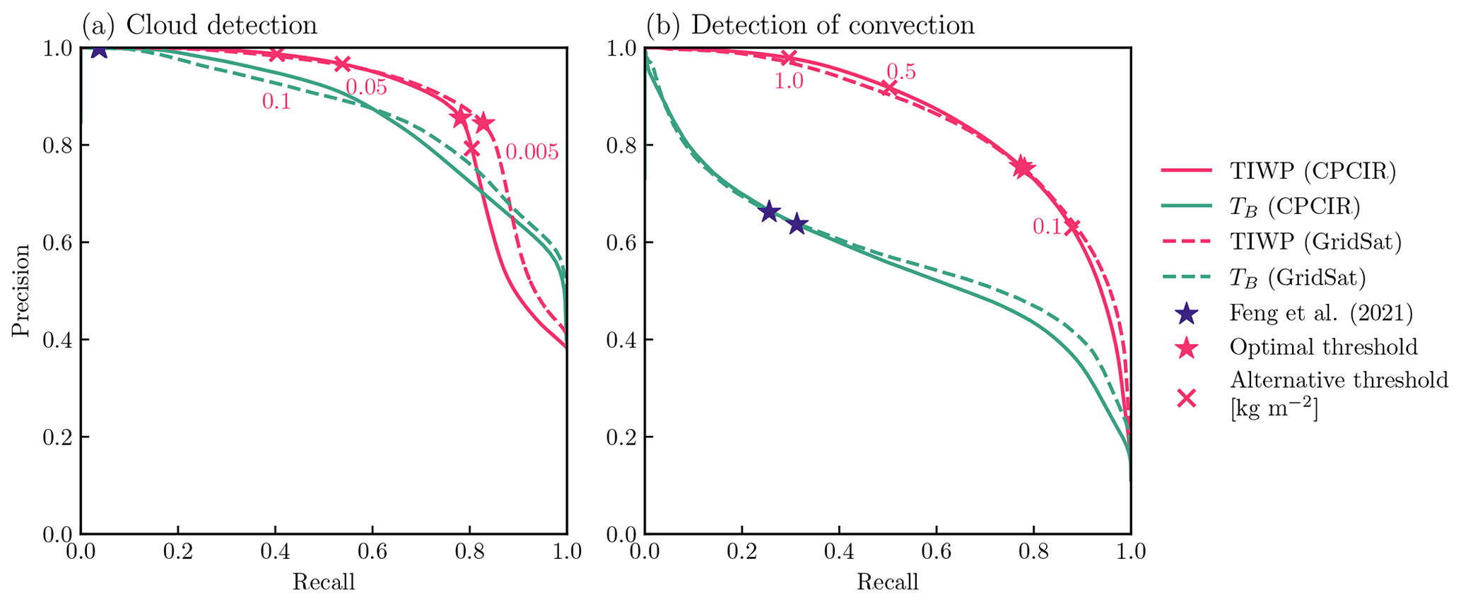
Figure 22 Precision–recall curves for the detection of clouds and convection using IR brightness temperatures and CCIC TIWP estimates for the test set. Panel (a) assesses the ability of the two quantities to identify cloudy 2B-CLDCLASS columns. The blue stars mark resulting performance of the 241 K threshold used by Feng et al. (2021) to identify cold cloud shields for the CPCIR and GridSat datasets. The pink stars mark the optimal decision threshold determined as the points closest (in terms of Euclidean distance) to a precision and recall of 1. The corresponding threshold values are 0.009 kg m⁻² for the CPCIR dataset and 0.012 kg m⁻² for GridSat. Additional markers show precision and recall for selected, additional TIWP detection thresholds. Panel (b) shows the same results for the detection of convective clouds (Cu, Nb, or deep convection) anywhere in the column. The blue stars mark the classification accuracy of the 225 K threshold used by Feng et al. (2021) to identify convective cores. The optimal threshold values for CPCIR and GridSat datasets are 0.18 and 0.16 kg m⁻², respectively.

The TIWP offers slightly better detection skill for detecting clouds; however, this is mostly limited to the region where the precision is around 0.8. For comparison, the global database by Feng et al. (2021) uses a threshold of 241 K to identify cold cloud shields. Since this value is relatively low and unlikely to be produced by anything other than a cloud, the threshold achieves a precision very close to 1 but only a very low recall, indicating that it misses a large number of clouds. Larger differences between the brightness temperatures and TIWP are found for the identification of convective cores. Here the TIWP offers a significant advantage compared to the brightness temperature threshold of 225 K used by Feng et al. (2021). A detection threshold of TIWP > 0.18 kg m⁻² yields slightly higher precision and a recall that is more than 2 times as high as when brightness temperatures are used.

A comparison of the identified clouds for the case study depicting the midlatitude cyclone shown in Fig. 5 is presented in Fig. 23. As these results show, the brightness temperature thresholds fail to identify any of the convective clouds identified by CloudSat. Moreover, the identified cloud field is discontinuous and fails to reproduce the structure of the cyclone. The TIWP-based classification identifies clouds more reliably and better reproduces the structure of the cyclone but overestimates the extent of the convective clouds associated with the cold front. Overall, the TIWP-based classification provides a better representation of the cloud systems associated with the cyclone that is in fairly good agreement with the general understanding of cloud processes occurring in frontal zones. Moreover, we note that the overestimation of convective regions may be balanced by choosing a higher detection threshold that would achieve a lower recall but higher precision, as exemplified by the dashed and dotted contours in Fig. 23.

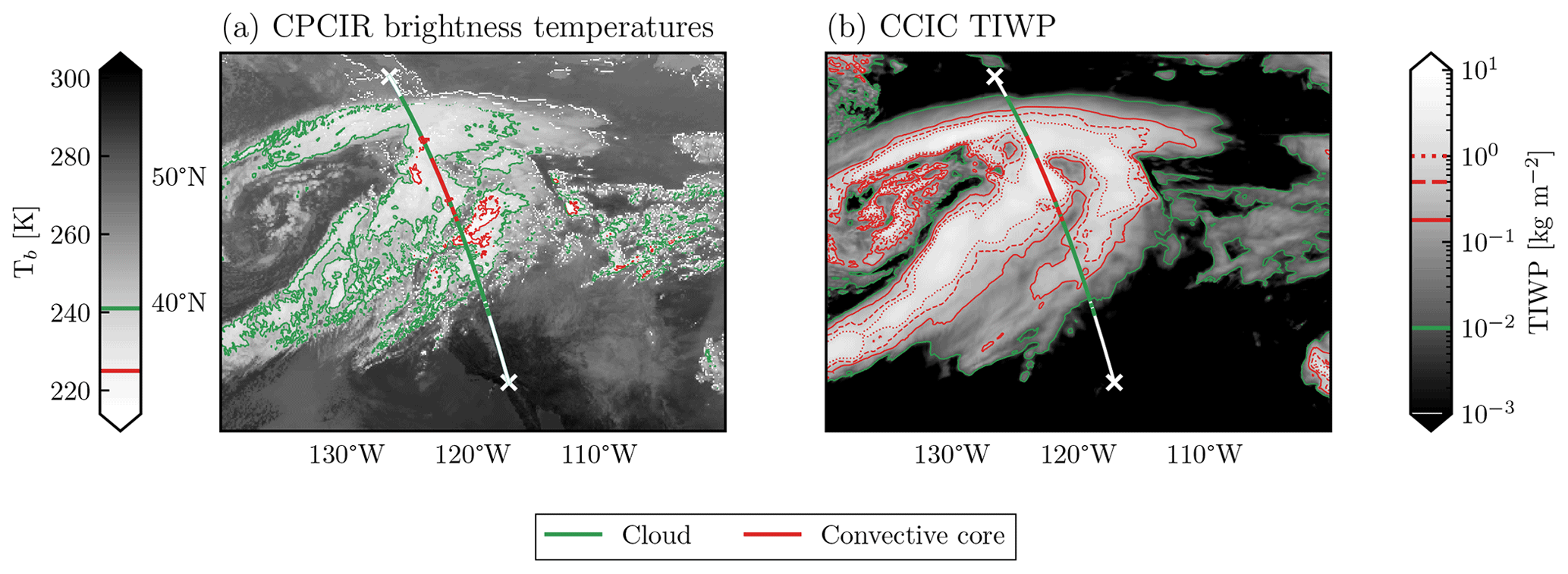
Figure 23 Cloud and convective regions as identified in brightness temperatures and TIWP for the midlatitude cyclone shown in Fig. 5. Panel (a) shows the identified regions based on the brightness temperature thresholds used in Feng et al. (2021) together with classes identified along the CloudSat overpass. Panel (b) shows the corresponding regions identified based on TIWP. Solid lines show regions resulting from the optimal detection thresholds identified in Fig. 22. Dashed and dotted lines show convective regions identified for higher detection thresholds of TIWP > 0.5 kg m⁻² and TIWP > 1.0 kg m⁻², respectively.

Since the issues of brightness-temperature-based cloud tracking are well known, Feng et al. (2021) and most other cloud-tracking approaches incorporate additional data such as precipitation estimates. Nonetheless, the results shown in Fig. 23 indicate that the features identified in brightness temperature fields may not provide a good representation of actual cloud systems. The retrieved TIWP fields directly estimate the concentration of ice particles in clouds and therefore provide a more direct signal to identify clouds than the IR brightness temperatures. Furthermore, high TIWP values are likely more directly related to convection than high cloud tops alone. This reasoning together with the results shown in Fig. 23 suggests that cloud tracking on TIWP likely provides a better representation of actual cloud systems than brightness-temperature-based tracking.

5.3.2 Climate studies and model assessment

Compared to raw brightness temperatures, TIWP has the advantage of being directly comparable to physical quantities represented in weather and high-resolution climate models. This should, at least in principle, simplify the identification of shortcomings in the representation of clouds.

Furthermore, the presented validation results show that CCIC can reliably characterize the spatial and temporal distribution of TIWP. This is in contrast to most other available observational TIWP datasets, which in most cases have much more limited spatial and temporal coverage and cannot constrain the full diurnal cycle of TIWP. Therefore, we see great potential for the CCIC data to provide novel insights into cloud processes. Finally, the CCIC data are provided at the same temporal resolution and coverage as many commonly used gridded precipitation products. The combination with precipitation estimates, in particular, may help to better constrain cloud and precipitation processes in models.

5.4 Data dissemination

With the conclusion of this validation study, we plan to begin the processing of the CCIC climate data record with the aim of publishing data records for the full temporal extent of the CPCIR and GridSat dataset. However, we will likely not be able to publish vertically resolved retrieval targets due to storage restrictions. To make these retrievals available for interested researchers, we publish the CCIC retrieval as a Python software package (Amell and Pfreundschuh, 2023). The software package provides a simple command line interface that will allow users to run the retrievals on their own hardware: a high-level description is provided in Appendix D. Information on how to access the latest processed climate data record is available through the software package repository at https://github.com/see-geo/ccic (last access: 19 April 2024).

6 Conclusions

This study presented and evaluated the CCIC hydrometeor retrieval, which aims to provide a new climate record of ice clouds based on the long record of geostationary IR observations. CCIC leverages novel deep-learning-based retrieval techniques to provide accurate estimates of concentrations of frozen hydrometeors and related cloud properties with spatially and temporally continuous coverage between 70° S and 70° N. The retrieval has been thoroughly characterized using 1 year of collocations with CloudSat 2C-ICE and 2B-CLDCLASS measurements and validated against independent measurements of TIWC and TIWP from two flight campaign series and a ground-based cloud radar. Albeit not achieving equally high spatial resolution as the CloudSat reference measurements, the retrieval provides reasonable accuracy in comparison with CloudSat and is consistent with the field campaign and ground-based radar measurements. Retrieval biases were found to be within ±60 % for a large number of in situ measurements in both tropical and midlatitude regimes. The CCIC retrievals are capable of reproducing the diurnal cycle of TIWP as measured by a ground-based radar, which shows that CCIC retrieval ideally complements currently available measurements from CloudSat and the A-Train, which are much more limited in the spatial and temporal coverage.

An important question that remains to be answered is the stability of the climate record across the full range of the input datasets, which we will address in a follow-up study. Nonetheless, the validation experiments presented here cover a long time range outside the time period that has been used for the training of the retrieval, which provides preliminary evidence of the stability of the retrieval. This makes us confident that the CCIC climate record will be a valuable addition to the currently available record of ice cloud properties and hopefully help to improve the understanding of cloud processes in the atmosphere.

Appendix A: Training set distributions

The probability distribution functions (PDFs) of brightness temperature, TIWP, and TIWC in the training set are given in Figs. A1, A2, and A3, respectively. Table A1 shows the frequencies of cloud classes and cloudy reference profiles.

Figure A1 Distribution of the brightness temperature closest to 11 µm in the training set.

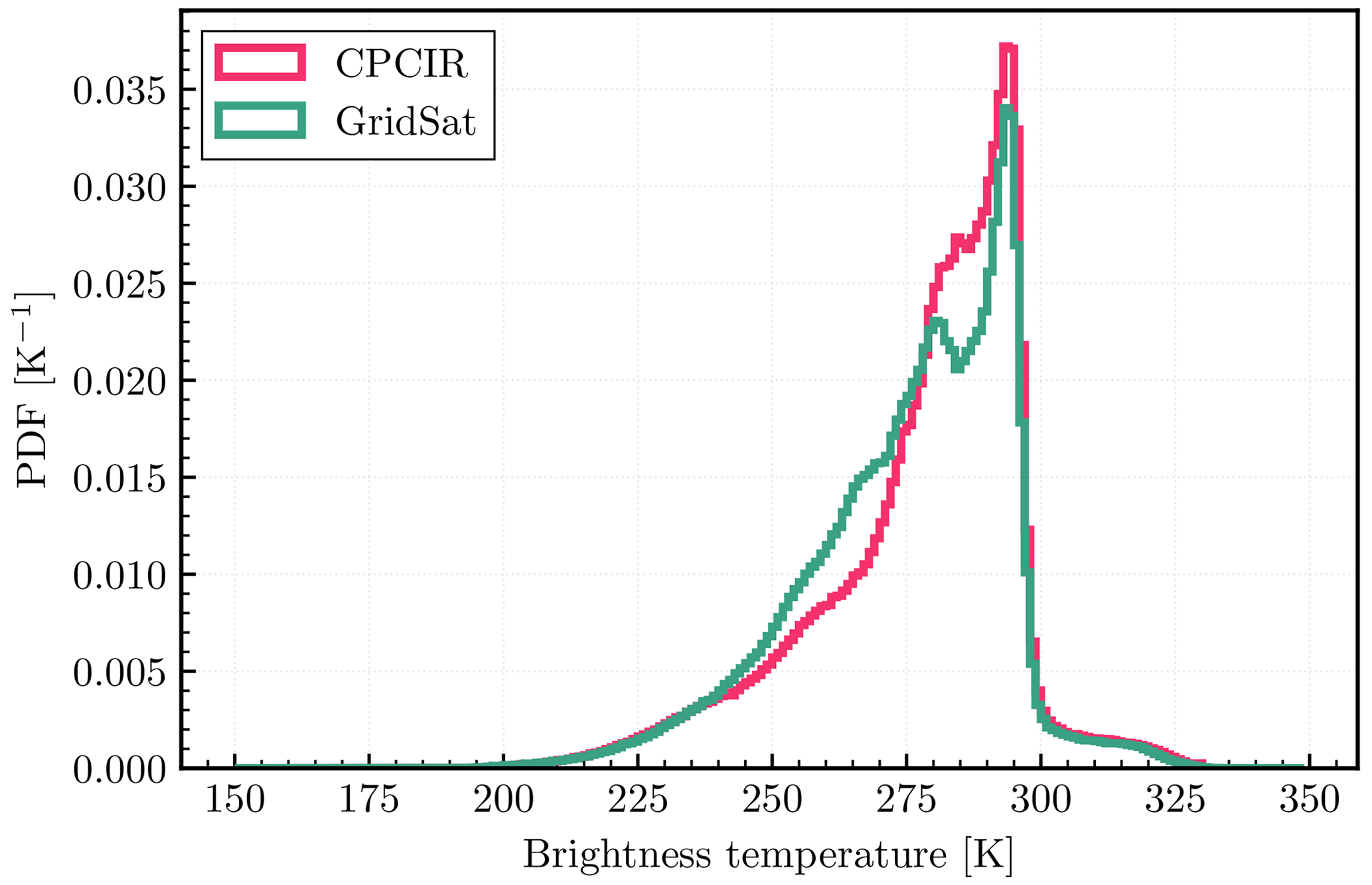
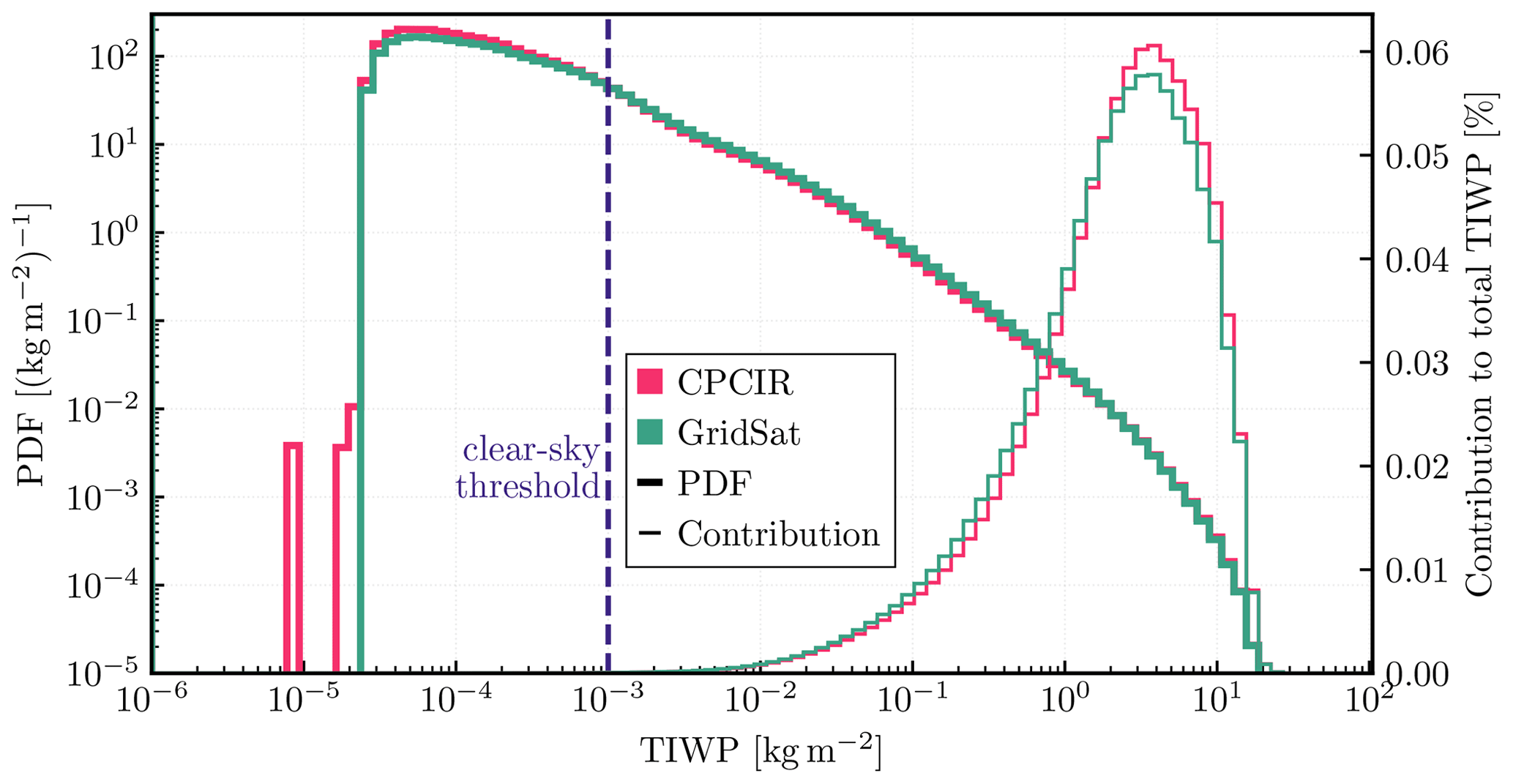
Figure A2 TIWP distributions in the training set. Probabilities of TIWP < 10⁻⁶ kg m⁻² for CPCIR and GridSat: 53.6 % and 50.8 %, respectively. Clear-sky threshold explained in Sect. 2.1.4.

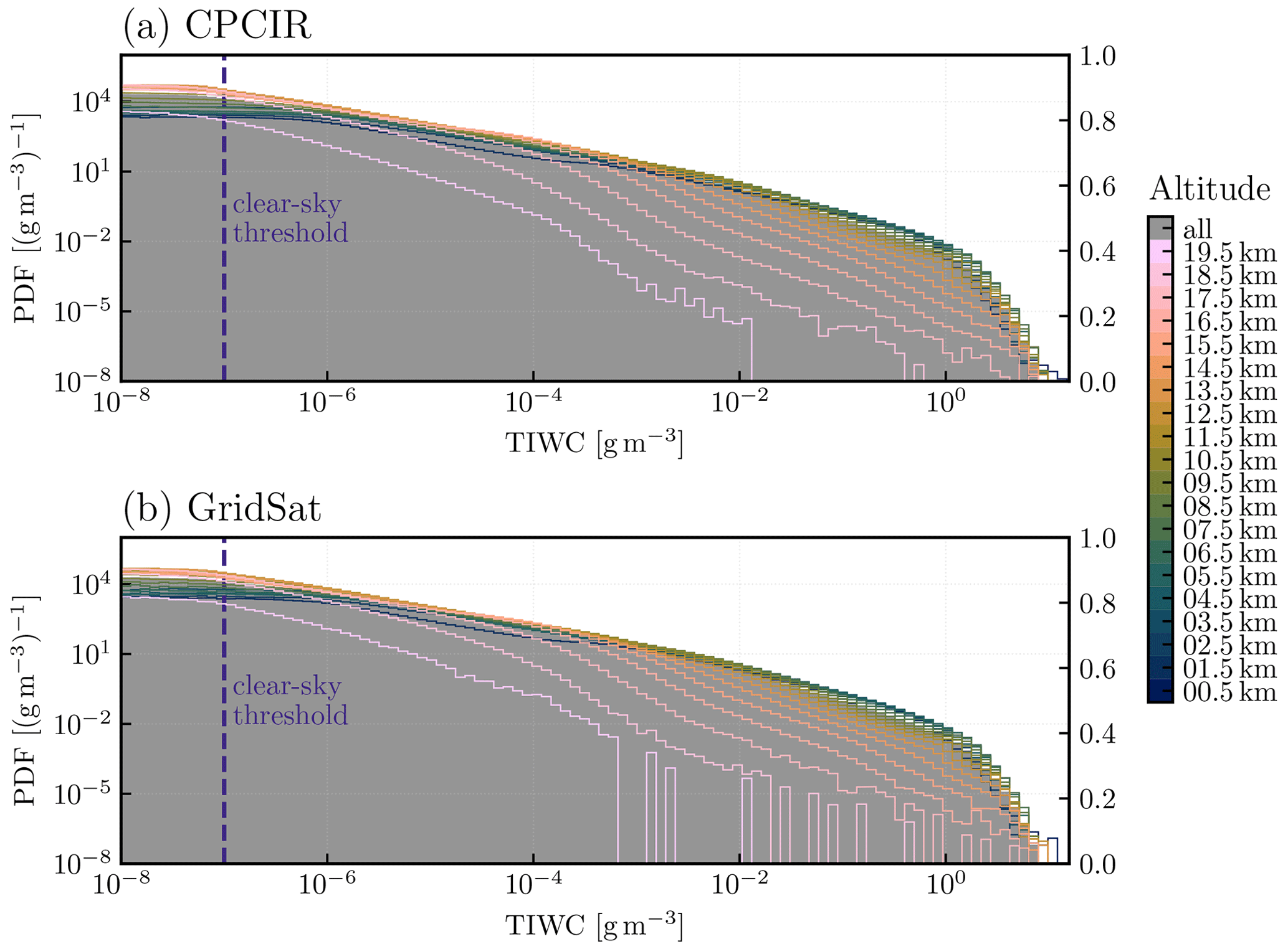
Figure A3 TIWC distributions in the training set at the different altitudes. Probabilities of TIWC < 10⁻⁸ g m⁻³ for CPCIR and GridSat for all altitude levels: 84.3 % and 83.3 %, respectively. Clear-sky threshold explained in Sect. 2.1.4.

Table A1 Cloud class frequencies, in percent, from all levels in the training set and total fraction of cloudy profiles, defined as a profile with at least one cloudy level.

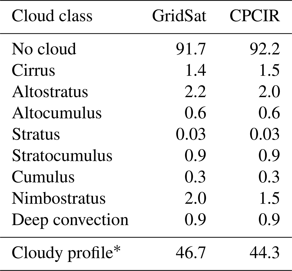
^* According to the 2D cloud mask.

Appendix B: Training settings

Table B1 shows training choices not mentioned in Sect. 2.1.4. Any parameter not specified corresponds to the default values in PyTorch 1.13.0 (Paszke et al., 2019b).

Table B1 Training choices not mentioned in text.

Appendix C: Radar retrievals

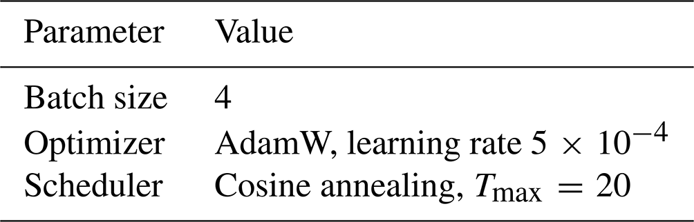
In order to compare CCIC retrievals with observations from airborne and ground-based cloud radar observations in a consistent manner, we have developed a radar-based TIWC retrieval based on the retrievals used in Pfreundschuh et al. (2022b). The input of the retrieval is range-resolved radar reflectivity measurements from which hydrometeor concentrations are derived using the optimal estimation method (OEM; Rodgers, 2000). The retrieval is implemented using the Atmospheric Radiative Transfer Simulator (ARTS; Buehler et al., 2018).

C1 Forward model

The ARTS-based radar forward model calculates polarized single-scattering radar reflectivities taking into account absorption from gases and particles. Gaseous absorption is modeled in the same way as described in Pfreundschuh et al. (2022b). Particle size distributions of frozen hydrometeors are represented using the single-moment parametrizations by Field et al. (2007). For liquid hydrometeors the parametrization by Abel and Boutle (2012) is used. The forward model assumes hydrometeors below the freezing level to be liquid and frozen above. The model will thus misrepresent melting particles and liquid particles in convective cores, which will incur an error in the retrieved hydrometeor concentrations.

Particle single-scattering properties are taken from the ARTS single-scattering database (SSDB; Eriksson et al., 2018). Since the assumed shape of ice particles represents a major source of uncertainty for radar-based retrievals of ice concentrations, we have selected a set of three particles that aim to capture the range of scattering properties in the ARTS SSDB. The particle models used are the eight-column aggregate, large-plate aggregate, and large-column aggregate, which are also used in the retrievals presented in Pfreundschuh et al. (2022b).

Atmospheric temperature, humidity, and liquid cloud water content are taken from ERA5 (Hersbach et al., 2020).

C2 HAIC-HIWC

During the Darwin leg of the HAIC-HIWC campaign, the RASTA (Radar Airborne System Tool for Atmosphere) was flown on board the F20 aircraft of the Service des Avions Français Instrumentés pour la Recherche en Environnement (SAFIRE) research aircraft. The RASTA system comprises multiple radar beams and measures Doppler spectra of radar reflectivity. For the retrievals used here, only total reflectivity from the zenith and azimuth beams was used in the retrieval. Input observations were resampled to a temporal resolution of 30 s and a vertical resolution of 100 m. The retrievals for the zenith and azimuth beams are performed independently. The retrievals used the PSD parametrization for tropical regimes by Field et al. (2007).

The radar retrievals from the HAIC-HIWC campaign are evaluated against in situ measurements in Fig. C1. The in situ measurements were performed by the same aircraft. The radar-retrieved TIWC at the aircraft position was obtained by linear interpolation between the TIWC retrieved 250 m above and 250 m below the aircraft. The radar retrievals are highly correlated with the in situ measurements for all particle models. The eight-column aggregate and large-plate aggregate models underestimate the TWC measured in situ. The large-column aggregate slightly overestimates the in situ measurements but yields results closest to the in situ measurements. The mean profiles of the logarithmic ratio of retrieved and in situ TWC indicate that the large-column aggregate and to a lesser degree also the large-plate aggregate yield relatively higher TIWC at lower altitudes.

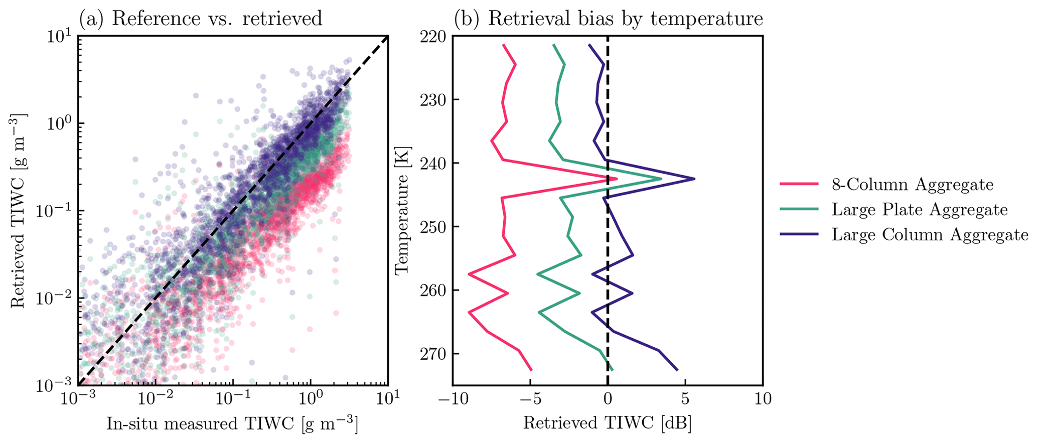
Figure C1 Comparison of radar retrievals and in situ measurements. Panel (a) displays the relation between retrieved TIWC and in situ measurements collocated at the spatial and temporal resolution of the CPCIR-based CCIC retrievals. Panel (b) displays the mean profiles of the logarithmic ratio of retrieved and in situ TIWC with respect to the atmospheric temperature.

Table C1 lists the correlation and mean biases of the radar retrieval and the in situ measurements. The retrieval bias is largest for the eight-column aggregate, which underestimates the mean TIWC by a factor of 4. For the large-plate aggregate the mean TIWC is underestimated by a factor of 2. The large-column aggregate yields the best agreement with the in situ measurements.

Table C1 Correlation and mean bias for different particle shapes assumed in the radar retrievals from the HAIC-HIWC campaign.

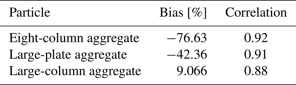
C3 OLYMPEX

During the OLYMPEX campaign, W-band cloud radar observations were conducted by the cloud radar system (CRS) on board the NASA ER-2 aircraft. The retrievals used the PSD parametrization for midlatitude regimes by Field et al. (2007). Figure C2 shows scatter plots of our CRS TIWC retrievals and collocated in situ measurements from the UND Citation aircraft. To collocate the radar and in situ measurements, both were mapped to the spatial and temporal resolution of the CCIC CPCIR retrieval.

Table C2 lists the mean bias of the radar retrieval and its correlation with the in situ measurements. The eight-column aggregate yields the best agreement with the in situ measurements. The large-plate and the large-column aggregate particle models overestimate the in situ measurements by 118 % and 344 %, respectively. Despite being lower than for the HAIC-HIWC, the retrieved TIWC remains well correlated with correlations between 0.73 and 0.74 for all particles.

Table C2 Correlation and mean bias for different particle shapes assumed in the radar retrievals from the OLYMPEX campaign.

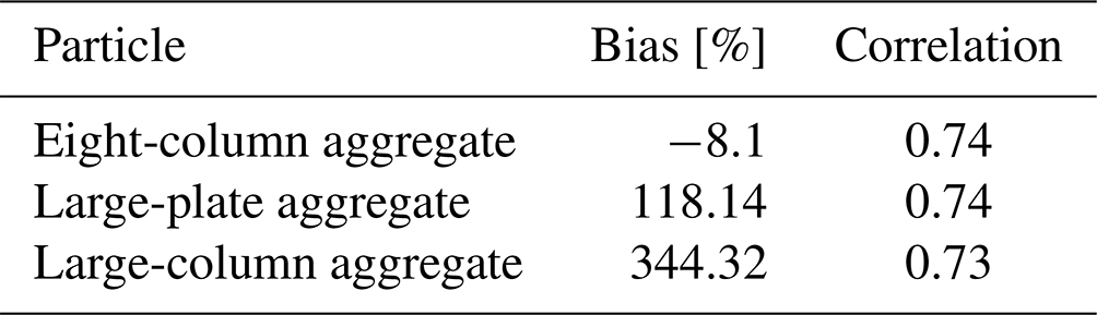
For the OLYMPEX campaign, the eight-column aggregate yields the best agreement with the in situ measurements. The large-plate and the large-column aggregate models both overestimate the TIWC. However, compared to the CCIC retrievals, the large-plate aggregate was found to yield biases that were more consistent with the biases between CCIC retrieval and in situ measurements. Since most collocations between the CRS radar and the UND in situ measurements stem from a single flight, we suspect that the inconsistency of the results in Fig. C2 and the comparison to the CCIC retrievals is due to the limited number of collocations of radar retrievals and in situ measurements and therefore choose the results obtained with the large-plate aggregate as the reference results for the OLYMPEX campaign.

C4 Cloudnet Palaiseau

The retrievals for the ground-based W-band cloud radar at the Cloudnet site in Palaiseau use the same retrieval framework as for the airborne radars. Radar reflectivities were averaged over 30 s and sampled at 4 min intervals. Retrievals were run for every day of the year 2019.

No in situ measurements were available to validate the ground-based radar retrievals. However, since retrievals with the large-plate aggregate were found to be consistent with CCIC and in situ retrievals for the OLYMPEX campaign, we chose the large-plate aggregate as the reference particle model.

Figure C2 Same as Fig. C1 but for the measurements from the OLYMPEX campaign.

Appendix D: The CCIC software package

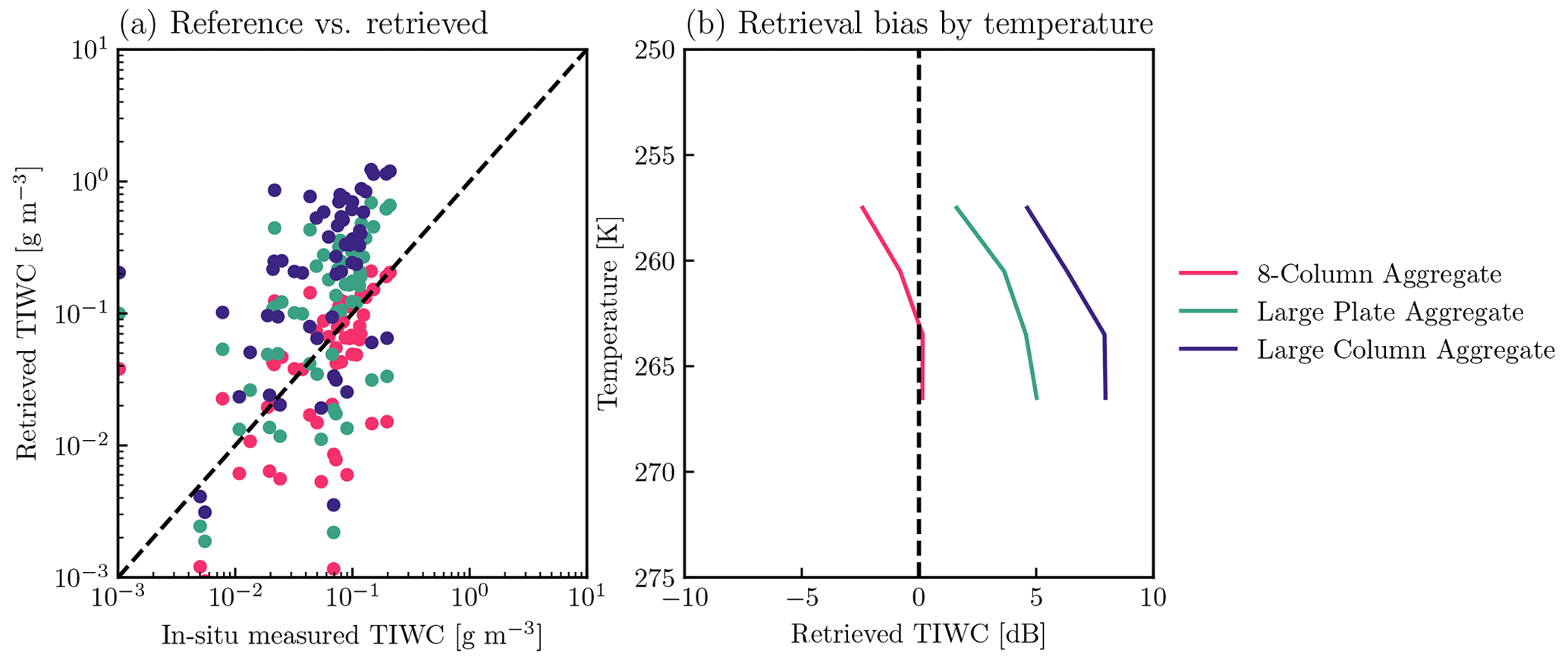
The NN developed and trained for CCIC is publicly available through the CCIC software package (Amell and Pfreundschuh, 2023), which facilitates running the retrievals on any modern computer. Given the fully convolutional NN nature of the CCIC NN, retrievals for small regions of interest (ROIs) are possible. The retrieval for large areas is implemented by dividing the input image in tiles that partly overlap, running the retrieval for each of these tiled areas, and finally aggregating the retrievals with a weighted average with weights inversely proportional to the distance to the center of each tile. This implementation aims to reduce the memory footprint of the inference and minimizes any CNN edge effects.

The software enables the user to choose, among others, a ROI, the variables of interest, and a CI complementing the TIWP expected value. The infamous quantile crossing problem (lack of monotonicity in the QPD) was detected in the retrieval of continuous variables, but, as discussed in Appendix E, it was deemed negligible for the default setting of a 90 % CI. Input data with invalid pixels are supported, since the CCIC NN likely leverages contextual information to provide a retrieval. Finally, the CCIC software package saves the retrievals either as compressed netCDF files or as Zarr files. The latter file format facilitates distributed access as well as significantly reduces the file size through a custom compression algorithm. Regardless of the file format used, the climate and forecast (CF) conventions (Eaton et al., 2022) are followed.

Appendix E: Is quantile crossing a problem for CCIC?

One of the properties that any cumulative distribution function (CDF) must have is to be a right-continuous monotone increasing function. With the formulation of QRNNs used, there is the possibility that the QPDs obtained violate this statistical property: for example, the quantile $x_{{\mathit{\tau }}_i}$ at level τ_i being larger than the quantile $x_{{\mathit{\tau }}_{i+\mathrm{1}}}$ at level ${\mathit{\tau }}_{i+\mathrm{1}}>{\mathit{\tau }}_i$, yet this would imply that ${\mathit{\tau }}_{i+\mathrm{1}}<{\mathit{\tau }}_i$. This is an infamous problem referred to as quantile crossing and arises from quantile regression itself. Depending on the formulation of the problem, it cannot be avoided: a minimal example is doing linear quantile regression for two levels for a cloud of points in ℝ². In this case, the lines obtained will extremely likely cross on the real line. Therefore, quantile crossing can require additional analysis or caution when drawing conclusions.

Inference with the GridSat training data for June 2006 is used here to analyze the presence and implications of quantile crossing for the retrievals offered by the CCIC software package, using a 90 % CI. The Spearman correlation coefficient ${\mathit{\rho }}_{\mathrm{S}}\in [-\mathrm{1},+\mathrm{1}]$ measures the monotonic relationship between two variables, with ±1 indicating a perfect monotonic relationship. Consequently, it can be used to assess the deviation of a QPD from a monotone function, i.e., the presence and magnitude of quantile crossing by computing ρ_S between the estimated quantiles and the quantile levels. This correlation results in ρ_S≥99.8 % for TIWP and ρ_S≥80.6 % for TIWC for all retrievals; these results are consistent with the argument that the retrieval of TIWC is more difficult. These high ρ_S values indicate that the QPDs are generally close to being perfect monotonic functions, but not all of them. However, these last QPDs can be considered to be relatively rare, as the median of the distributions of ρ_S for any of the three variables is practically 1.

There are numerous approaches to address quantile crossing. An option is to process the QPD with a linear isotonic regression of the quantiles x_τ by solving

$$\begin{array}{}\text{(E1)}& \begin{array}{ll}\text{minimize}& {\sum }_{{\mathit{\tau }}_i\in \mathcal{T}}{\left(x_{{\mathit{\tau }}_i}^{\left(c\right)}-x_{{\mathit{\tau }}_i}\right)}^{\mathrm{2}}\\ \text{subject to}& x_{{\mathit{\tau }}_i}^{\left(c\right)}\le x_{{\mathit{\tau }}_j}^{\left(c\right)}\forall {\mathit{\tau }}_i\le {\mathit{\tau }}_j\end{array}\end{array}$$

and obtaining quantiles $x_{\mathit{\tau }}^{\left(c\right)}$ that are monotonic. The idea behind this approach is to have a simple, computationally friendly method that respects as much as possible the QPD given by the network. Figure E1 shows the QPDs with the worst ρ_S for the “tiwp” and “tiwc” variables, as well as the corrected QPDs (CQPDs) through a linear isotonic regression. At least three things can be spotted in Fig. E1: the highly nonlinear shape of the QPDs, the quantile levels with crossing quantiles, and that the QPD and CQPD expected values are virtually identical. Intuitively, nearby quantile levels have higher odds of experiencing quantile crossing than distant levels. Consequently, a large CI is more robust: all quantiles defining the 90 % CI for the retrievals analyzed do not cross.

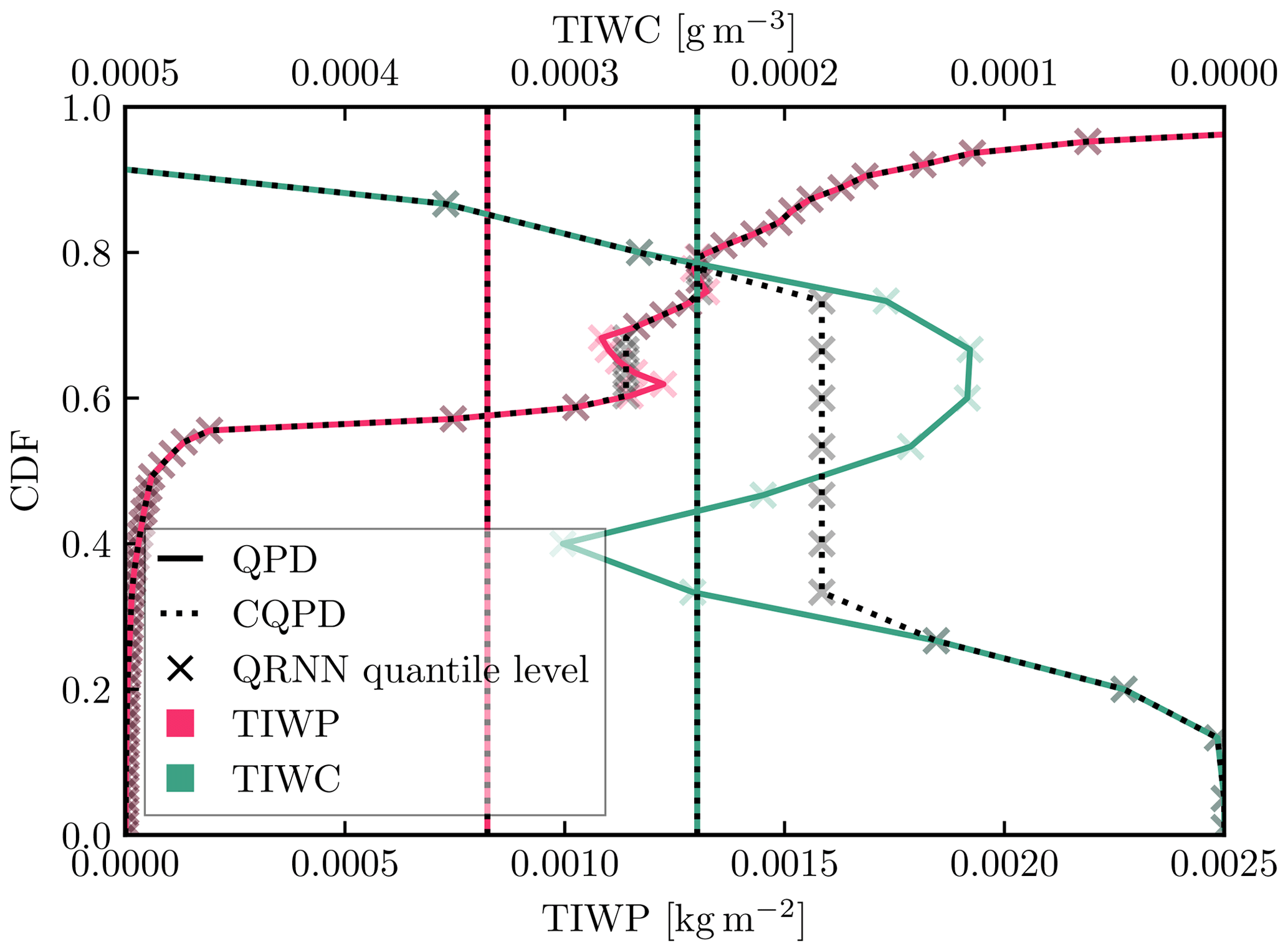
Figure E1 QPDs with the worst ρ_S (99.8 % for TIWP and 80.6 % for TIWC), where the vertical lines indicate the expected value of the corresponding distribution. Note the different abscissa axes and that the plot limits were deliberately selected to draw attention to the crossing quantiles.

Computing the signed relative percent difference between a scalar x derived from the QPD and the analogous value derived from the CQPD, referred as x^(c), enables comparison among different orders of magnitude. In this analysis their mean is used as a reference, i.e.,

$$\begin{array}{}\text{(E2)}& d_{\mathrm{1}}(x,x^{\left(c\right)})={\displaystyle \frac{x-x^{\left(c\right)}}{\left(\left|x\right|+\left|x^{\left(c\right)}\right|\right)/\mathrm{2}}},\end{array}$$

with $d_{\mathrm{1}}(\mathrm{0},\mathrm{0})=\mathrm{0}$, and therefore ranges from −2 to +2. The distribution of d₁ values for all TIWP and TIWC variables resembles a delta function, with 99 % of the values being zero and the quantiles defining the 99.9 % equal-tailed distribution for TIWP-derived ρ_S being −0.0011 and 0.0151. Consequently, there may be instances of quantile crossing, but its impact on the variables reported by the CCIC software package is negligible when contrasted with enforcing monotonicity of the QPDs through linear isotonic regression.