Improving the estimate of higher-order moments from lidar observations near the top of the convective boundary layer

Ground-based lidar data have proven extremely useful for profiling the convective boundary layer (CBL). Many groups have derived higher-order moments (e.g., variance, skewness, fluxes) from high-temporal-resolution lidar data using an autocovariance approach. However, these analyses are highly uncertain near the CBL top when the depth of the CBL (z_i) is changing during the analysis period. This is because the autocovariance approach is usually applied to constant height levels and the character of the eddies is changing on either side of the changing CBL top. Here, a new approach is presented wherein the autocovariance analysis is performed on a normalized height grid, with a temporally smoothed z_i. Output from a large eddy simulation model demonstrates that deriving higher-order moments from time series on a normalized height grid has better agreement with the slab-averaged quantities than the moments derived from the original height grid.

1 Introduction

The atmospheric boundary layer (ABL) is the lowest portion of the atmosphere, typically ranging in depth from 10 m in extremely stable conditions to over 3 km, that interacts directly with the surface and is responsible for the majority of our weather (Stull, 1988). In particular, the ABL often has significant variability over the diurnal cycle due to the changing net radiation at the surface caused by the solar cycle. During the day when the surface is being heated by the sun, turbulent eddies rising from the surface create a well-mixed convective boundary layer (CBL) with turbulent eddies that range from approximately the size of the depth of the CBL (which will be denoted here as z_i) to sub-meter in size. Understanding and characterizing the properties of this turbulent CBL is critical to improving the modeling of transport and mixing within the CBL in weather and climate models (Deardorff, 1974; Wilde et al., 1985).

Observations of turbulent mixing have been made for many dozens of years. Today's technologies include rapid response sonic anemometers and gas analyzers for in situ observations, scintillometers for open-path observations over larger volumes, and lidar observations from which profiles of turbulent moments can be derived. Higher-order moments, such as the variance and skewness of a scalar, as well as covariances between two geophysical variables (e.g., water vapor and vertical motion), are used to describe the turbulence in the CBL statistically. There are multiple areas where better understanding of these higher-order moments is useful. For example, moisture variance in the CBL is important for understanding the boundary layer moisture budget (Deardorff, 1974; Lenschow and Wyngaard, 2014; Huang et al., 2011), the development of boundary layer clouds (Wilde et al., 1985; Golaz et al., 2002; Berg et al., 2005), and the development of deep convection (e.g., Berg et al., 2013). Indeed, Wulfmeyer et al. (2016) outlined a powerful approach that could be used to evaluate a wide range of similarity relationships that relate vertical gradients and mean profiles to turbulent moments using advanced ground-based lidar observations; similarity relationships often form the basis of turbulent parameterizations used within mesoscale and climate models.

Here, we focus on lidar observations of turbulent moments within the CBL. Lidar observations of water vapor (e.g., Muppa et al., 2016; Turner et al., 2014), temperature (Behrendt et al., 2015), vertical motions (Berg et al., 2017; Lenschow et al., 2012), aerosols (McNicholas and Turner, 2014), and fluxes (Behrendt et al., 2020; Kiemle et al., 2007; Senff et al., 1994) have been used to derive higher-order moments in various locations. Lidar data, however, are frequently noisy due to both changing solar contributions and instrument noise, and thus separating out the atmospheric component to the higher-order moments from the noise is challenging. Most lidar groups analyzing higher-order moments use the autocovariance technique pioneered by Lenschow et al. (2000) (hereafter, L-2000) to separate the two contributions, wherein the moments at lags above zero, which do not have any contribution from the instrument error, which is assumed to be uncorrelated with time, are interpolated back to lag 0.

The L-2000 approach assumes that the turbulent nature of the CBL does not change with time since statistics are derived from high-temporal-resolution time series, given that the lidars are most often measuring very small volumes in the vertical column above and below the lidar. Furthermore, as the larger eddies carry the most energy yet also occur less frequently, the time window analyzed must be sufficiently long to reduce the sampling uncertainty (Lenschow et al., 1994; hereafter, L-1994). The two constraints provided by L-1994 and L-2000 restricts the analysis of lidar data to 1–2 h periods when the CBL is quasi-stationary (i.e., where z_i is not changing with time); these conditions are most commonly found in the mid to late afternoon (e.g., from 15:00 to 17:00 CDT (central daylight time) in Fig. 1).

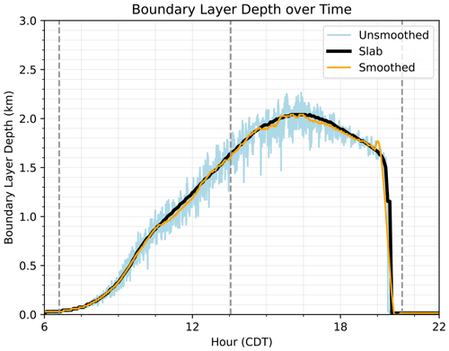
Figure 1 CBL depth over time, derived from the slab values (black, $<z_i\left(t\right)>$), the instantaneous 10 s values of a single column (blue, z_c,i(t)), and the 60 min temporal average of the instantaneous values of the single column (orange, $\stackrel{\mathrm{‾}}{z_{\mathrm{c},i}\left(t\right)}$).

However, there is a strong desire to be able to derive higher-order moments from lidar observations when the CBL is rapidly evolving, such as the time period after the morning transition to when the CBL stops growing (e.g., from 10:00 to 15:00 CDT in Fig. 1). Some studies have derived higher-order moments from lidar data during periods when z_i is rapidly changing; this is often done by restricting the analysis to shorter time periods to derive the statistics (e.g., the 30 min window used in Berg et al., 2017), which results in larger sampling uncertainties (per L-1994). Furthermore, all of these analyses are done on a fixed height grid; i.e., the higher-order moments are derived by looking at the time series at each range gate (height) observed by the lidar. This approach of using a fixed height grid from which to define the moments is insufficient at the top of the CBL when z_i passes through the height layer being analyzed (z_anal) during the analysis period (i.e., z_i < z_anal early in the period and z_i > z_anal at the end of the period).

This work presents a new approach (outlined in Sect. 2) to analyze lidar profile observations over time when the height of the CBL is changing over that time. The approach is simple: change the vertical coordinate from height to normalized height before computing the statistics over temporal windows. This paper demonstrates this approach using output from a large-eddy simulation model (Sect. 3), wherein we can use a single column to approximate the lidar observations and spatial statistics to serve as truth.

2 Approach

Our proposed approach is simple: instead of deriving higher-order moments on a fixed height grid (z), the data are transformed to a normalized height grid ($\widehat{z}=z/\stackrel{\mathrm{‾}}{z_i}$) where the overbar indicates a temporal average. The advantage of this scheme is as follows: if $\widehat{z}$ < 1 (> 1) for the entire analysis period, then it is known that the time series is entirely within (above) the CBL. This greatly simplifies the understanding of the statistics. The challenge thus becomes understanding the time period over which to derive $\stackrel{\mathrm{‾}}{z_i}$ and demonstrating that computing the moments on the $\widehat{z}$ grid is more accurate than using the regular z grid.

To investigate this, we utilized large-eddy simulations of the CBL. The simulation used the Department of Energy's Atmospheric Radiation Measurement (ARM) constrained variational analysis (VARANAL) for initial and boundary conditions (Xie, 2017). VARANAL yields values for surface fluxes, large-scale advective and radiative tendencies that are spatially averaged over the entire ARM Southern Great Plains (SGP) domain. These simulations were performed with the MicroHH model (van Heerwaarden et al., 2017), using 25 m horizontal spacing over a 10 km × 10 km domain and 15 m vertical resolution. Statistics output every 5 min and derived over the entire domain were used as truth, and the lidar data were simulated by extracting out a high temporal resolution (10 s) time series at a single location in the middle of the domain. For this work, we will show results from 8 August 2017 over the ARM program (Turner and Ellingson, 2016) SGP site (Sisterson et al., 2016). However, very similar results were found on other days, and these are not shown.

The evolution of the depth of the CBL (i.e., z_i) from the LES (large-eddy simulations), derived through three different methods, is shown in Fig. 1. All three methods compute z_i as the level of neutral buoyancy of a surface-based parcel, which we found as the first height index at each time where the potential temperature (θ) is a value δ greater than the first height level at that time, where δ is 0.5c_p. However, method 1 was derived from the slab-averaged output from the LES, yielding z_i at each time t (i.e., over the entire model domain); method 2 was the instantaneous z_i value for the selected column c (i.e., mimicking an instantaneous lidar observation) at time t; and method 3 used a third-order Savitzky–Golay filter with a 1 h window to temporally average z_i at that selected column c around time t. These will be denoted by $<z_i\left(t\right)>$, z_c,i(t), and $\stackrel{\mathrm{‾}}{z_{\mathrm{c},i}\left(t\right)}$, respectively. All three of these were derived as the level of neutral buoyancy, where the θ used for $<z_i\left(t\right)>$ was from the slab-averaged LES output, for z_c,i(t) it was the instantaneous θ from an individual column, and for $\stackrel{\mathrm{‾}}{z_{\mathrm{c},i}\left(t\right)}$ it was the temporally averaged z_c,i(t).

For this work, we computed time–height cross sections of variance, skewness, and kurtosis of water vapor mixing ratio (q) from the LES output using three approaches: (a) using spatial statistics at each height level, which served as the truth dataset; (b) the baseline approach for a single column, wherein the statistics were computed on a fixed z grid; and (c) the new approach for a single column where the statistics were computed on a normalized $\widehat{z}$ grid using $\stackrel{\mathrm{‾}}{z_{\mathrm{c},i}\left(t\right)}$, after which the moments were interpolated back to the regular z grid for comparison. We computed the variance and skewness at each level in the z or $\widehat{z}$ grid by first extracting out the time series at that level for the time period being analyzed and detrending it. The variance is then computed as

$$\begin{array}{}\text{(1)}& \text{Var}\left(q\right)={\displaystyle \frac{\mathrm{1}}{N}}\mathrm{\Sigma }{\left(q-\stackrel{\mathrm{‾}}{q}\right)}^{\mathrm{2}},\end{array}$$

the skewness as

$$\begin{array}{}\text{(2)}& \text{Skew}\left(q\right)={\displaystyle \frac{\mathrm{\Sigma }{\left(q-\stackrel{\mathrm{‾}}{q}\right)}^{\mathrm{3}}}{(N-\mathrm{1})\left(\text{Var}\right(q){)}^{\frac{\mathrm{3}}{\mathrm{2}}}}},\end{array}$$

and the kurtosis as

$$\begin{array}{}\text{(3)}& \text{Kurt}\left(q\right)={\displaystyle \frac{\mathrm{\Sigma }{\left(q-\stackrel{\mathrm{‾}}{q}\right)}^{\mathrm{4}}}{(N-\mathrm{1})\left(\text{Var}\right(q){)}^{\mathrm{2}}}},\end{array}$$

where N is the number of points in the analysis window.

Note that we did not use the L-2000 technique here, as we did not attempt to simulate a true lidar observation by superimposing any random error. The primary purpose of this study is to demonstrate that using the normalized $\widehat{z}$ grid provides more accurate measures of the variance, skewness, and kurtosis than using the regular z grid, even though the former includes a contribution from the interpolation error that was introduced by putting the data on the $\widehat{z}$ grid. Since the $\widehat{z}$ grid is a much finer resolution than the regular height grid, this interpolation error is extremely small.

3 Results

In each of the following contour figures, data above 1.2 z_i have been masked so that we can focus on the top of the boundary layer and below. Additionally, sunrise, noon, and sunset times are shown with dashed lines in the figures. A comparison of the q variance from the three calculation methods is shown in Fig. 2. The slab value results (left) are the truth to which the other two methods are compared. The slab values show that the variance is the highest at the top of the boundary layer from 10:00–17:30 CDT, after which it tapers off. Below the boundary layer top, the variance is much smaller. Both methods capture the higher variance along the top of the boundary layer, but the normalized $\widehat{z}$ grid has less of a gap just before 15:00 CDT, whereas the regular grid has a more significant gap at that point. Both methods are close to the slab values, except at 12:30 CDT and 15:00 UTC along the top of the boundary layer.

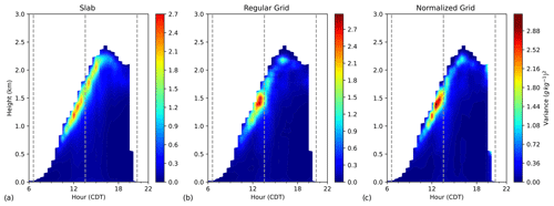
Figure 2 Time–height cross sections of q variance (units of (g kg⁻¹)²) computed from slab values at each height (a) on a regular z grid (b) and on the normalized $\widehat{z}$ grid (c). Both panels (b) and (c) are averaged over a 1 h period centered on each 30 min.

The q skewness is compared in Fig. 3. These figures clearly show that the normalized $\widehat{z}$ grid values are closer to the slab values in both magnitude and shape. Again, turning our attention to the values at the top of the boundary layer from 10:00–17:30 CDT, there is high skewness in a very thin layer. The regular grid underestimates the magnitude of the skewness here and overestimates the size of the layer with the highest skewness values. At the surface, both methods show higher levels of skewness than the slab at 15:00 CDT and beyond.

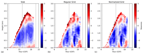
Figure 3 Time–height cross sections of q skewness (unitless) computed from slab values at each height (a) on a regular z grid (b) and on the normalized $\widehat{z}$ grid (c). Both panels (b) and (c) are averaged over a 1 h period centered on each 30 min.

In the case of latent heat flux, the different grid methods must be applied to both q and w. The results for the flux $\left(\stackrel{\mathrm{‾}}{q^{\prime }{w}^{\prime }}\right)$ are shown in Fig. 4. There are some clear differences between both grid methods and the slab values. The maximum flux is significantly higher than the slab values, and the two methods do not capture the flux well before 12:30 CDT, especially in the middle of the boundary layer.

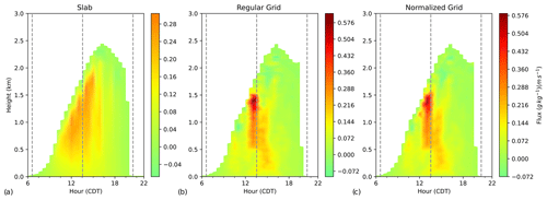
Figure 4 Time–height cross sections of latent heat flux $\left(\stackrel{\mathrm{‾}}{q^{\prime }{w}^{\prime }}\right)$ (units of g kg⁻¹(m s⁻¹)) computed from slab values at each height every 30 min (a) on a regular z grid (b) and on the normalized $\widehat{z}$ grid (c). Both panels (b) and (c) are averaged over a 1 h period centered on each 30 min.

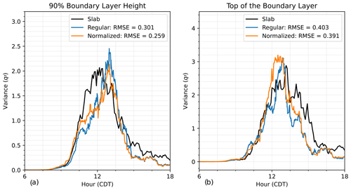
Figure 5 Line plot comparison of q variance (units of g kg⁻¹(m s⁻¹)) at 90 % of the boundary layer (a) and at the top of the boundary layer (b) for the three computation methods, i.e., slab (black), regular grid (blue), and normalized $\widehat{z}$ grid (orange), along with their respective root-mean-square error (calculated over the time period of 08:00–18:00 CDT) with respect to the slab value results.

To better quantify the differences between these two methods and the slab values, Figs. 5–7 show line plots of the variance (Fig. 5), skewness (Fig. 6), and latent heat flux (Fig. 7) at 90 % of the boundary layer (Figs. 5–7a​​​​​​​) and the top of the boundary layer (Figs. 5–7b) and their respective root-mean-square errors (RMSEs) calculated over the time window of 08:00–18:00 CDT. The RMSE is calculated based on the difference between each grid method and the slab values. We see that for the variance (Fig. 5) and at both depths that the normalized $\widehat{z}$ grid RMSE value is lower than the regular grid RMSE value, which shows that the normalized $\widehat{z}$ grid method better captures the variance towards the top of the boundary layer than the regular grid method. For the skewness (Fig. 6) at 90 % of the boundary layer (Fig. 6a) and the top of the boundary layer (Fig. 6b), the normalized grid method is significantly better than the regular grid method. Finally, looking at the flux (Fig. 7), the $\widehat{z}$ grid method yields slightly smaller RMSE values at 90 % of the boundary layer (Fig. 7a) and at the top of the boundary layer (Fig. 7b).

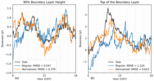
Figure 6 Line plot comparison of q skewness (unitless) at 90 % of the boundary layer (a) and at the top of the boundary layer (b) for the three computation methods, i.e., slab (black), regular grid (blue), and normalized $\widehat{z}$ grid (orange), along with their respective root-mean-square error with respect to the slab value results.

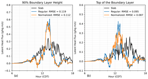
Figure 7 Line plot comparison of latent heat flux $\left(\stackrel{\mathrm{‾}}{q^{\prime }{w}^{\prime }}\right)$ (units of g kg⁻¹(m s⁻¹)) at 90 % of the boundary layer (a) and at the top of the boundary layer (b) for the three computation methods, i.e., slab (black), regular grid (blue), and normalized $\widehat{z}$ grid (orange), along with their respective root-mean-square error with respect to the slab value results.

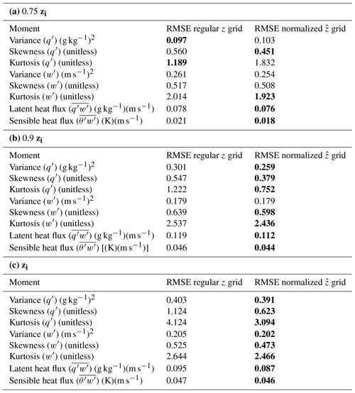
We extended these methods to the case of the fourth moment (kurtosis) and calculated the variance, skewness, and kurtosis of vertical velocity (w). Table 1a–c compare the RMSE values of the regular and normalized $\widehat{z}$ grid methods for calculating the variance, skewness, and kurtosis of q and w and the sensible $\left(\stackrel{\mathrm{‾}}{{\mathit{\theta }}^{\prime }{w}^{\prime }}\right)$ and latent heat fluxes $\left(\stackrel{\mathrm{‾}}{q^{\prime }{w}^{\prime }}\right)$ at various heights throughout the boundary layer (0.75z_i, 0.9z_i, and z_i). In this table, the grid method with the lower standard error for a given variable is bolded. We found that at 0.5z_i neither grid method stood out as better because the RMSE values were either effectively the same or better for an equal number of calculations, and thus we turn our attention to heights closer to the boundary layer depth. At 0.75z_i (Table 1a), the normalized $\widehat{z}$ grid method is better for every calculation except q variance and q kurtosis, where the regular grid method is better. For 0.9z_i (Table 1b), the normalized $\widehat{z}$ grid method is better in all cases except w variance, where the methods yield the same RMSE. Finally, at the top of the boundary layer (Table 1c), the normalized $\widehat{z}$ grid method is better in all cases. At every height, the normalized $\widehat{z}$ grid method was better for q skewness, w kurtosis, and both fluxes. At depths closer to the boundary layer depth, the importance of the normalized $\widehat{z}$ grid method for more accurate calculations becomes increasingly clear.

Table 1 Comparison of the root-mean-squared errors for the regular z grid and normalized $\widehat{z}$ grid methods calculated over the time window of 08:00–18:00 CDT at 0.75z_i, 0.9z_i, and z_i. Bolded values indicate RMSE values smaller than the other height grid by the standard error of the two.

4 Discussion

The normalized $\widehat{z}$ grid more accurately captures the q and w variance, skewness, kurtosis, and temperature and moisture fluxes, especially at heights approaching the top of the boundary layer. By accounting for changes in the boundary layer over time, this approach allows for a more accurate analysis of turbulence characteristics, particularly while the CBL is actively growing. This was particularly true for skewness, suggesting that higher-order moments would benefit more from this new approach. These results are consistent across multiple analysis days (not shown).

Previous work that only considers a regular grid could be reanalyzed to be more accurate with this method. In the future, this method can be used for more accurate lidar analysis of the CBL turbulent statistics during the late morning transition. A larger time window could be used since the changes in the boundary layer are already considered in the analysis, which will reduce the sampling uncertainty relative to previous studies done on a regular grid.

Further refinement is still necessary to determine optimal analysis periods guided by L-1994. Additionally, this method also would need to be adjusted for extremely rapid changes in z_i, such as during the evening transition. In cases where neither grid accurately captures the slab values, we must remember that a single column will never be able to properly capture the spatial variability because of sampling uncertainties. It is clear, especially in the q variance and latent heat flux time–height cross sections around 12:30 CDT, that the single column is experiencing an updraft that is not representative of the entire domain. Further work must be done to reduce the impact of spatial variability.

5 Conclusions

This work shows that using a normalized $\widehat{z}$ grid to calculate q and w variance, skewness, kurtosis, and temperature and moisture fluxes allows for a better representation of higher-order moments, especially at the top of the boundary layer, when compared to the higher-order moments and fluxes derived from the values over the entire domain. By transforming data to a normalized grid, we overcome limitations of the regular grid, particularly during the rapid growth of the CBL. This results in more accurate moments and is more impactful for higher-order (e.g., third-order) moments. This opens up the ability to describe these moments more accurately in a growing CBL, which will lead to improvements in modeling mixing in future climate and weather models.

In forthcoming work, we will discuss methods for handling spatial variability by determining optimum spacing and number of columns to represent a larger domain more accurately. Additionally, work needs to be done to determine optimum analysis periods and to refine the method for cases where the boundary layer depth is rapidly changing (e.g., during the evening transition).