the Creative Commons Attribution 4.0 License.
the Creative Commons Attribution 4.0 License.
 | 18 Feb 2021
Detection and quantification of CH4 plumes using the WFM-DOAS retrieval on AVIRIS-NG hyperspectral data
Jakob Borchardt
Konstantin Gerilowski
Sven Krautwurst
Heinrich Bovensmann
Andrew K. Thorpe
David R. Thompson
Christian Frankenberg
Charles E. Miller
Riley M. Duren
John Philip Burrows
Methane is the second most important anthropogenic greenhouse gas in the Earth's atmosphere. To effectively reduce these emissions, a good knowledge of source locations and strengths is required. Airborne remote sensing instruments such as the Airborne Visible InfraRed Imaging Spectrometer – Next Generation (AVIRIS-NG) with meter-scale imaging capabilities are able to yield information about the locations and magnitudes of methane sources. In this study, we successfully applied the weighting function modified differential optical absorption spectroscopy (WFM-DOAS) algorithm to AVIRIS-NG data measured in Canada and the Four Corners region. The WFM-DOAS retrieval is conceptually located between the statistical matched filter (MF) and the optimal-estimation-based iterative maximum a posteriori DOAS (IMAP-DOAS) retrieval algorithm, both of which were already applied successfully to AVIRIS-NG data. The WFM-DOAS algorithm is based on a first order Taylor series approximation of the Lambert–Beer law using only one precalculated radiative transfer calculation per scene. This yields the fast quantitative processing of large data sets. We detected several methane plumes in the AVIRIS-NG images recorded during the Arctic-Boreal Vulnerability Experiment (ABoVE) Airborne Campaign and successfully retrieved a coal mine ventilation shaft plume observed during the Four Corners measurement campaign. The comparison between IMAP-DOAS, MF, and WFM-DOAS showed good agreement for the coal mine ventilation shaft plume. An additional comparison between MF and WFM-DOAS for a subset of plumes showed good agreement for one plume and some differences for the others. For five plumes, the emissions were estimated using a simple cross-sectional flux method. The retrieved fluxes originated from well pads, cold vents, and a coal mine ventilation shaft and ranged between (155 ± 71) kg (CH4) h−1 and (1220 ± 450) kg (CH4) h−1. The wind velocity was a significant source of uncertainty in all plumes, followed by the single pixel retrieval noise and the uncertainty due to atmospheric variability. The noise of the retrieved CH4 imagery over bright surfaces (>1 µW cm−2 nm−1 sr−1 at 2140 nm) was typically ±2.3 % of the background total column of CH4 when fitting strong absorption lines around 2300 nm but could reach over ±5 % for darker surfaces (< 0.3 µW cm−2 nm−1 sr−1 at 2140 nm). Additionally, a worst case large-scale bias due to the assumptions made in the WFM-DOAS retrieval was estimated to be ±5.4 %. Radiance and fit quality filters were implemented to exclude the most uncertain results from further analysis mostly due to either dark surfaces or surfaces where the surface spectral reflection structures are similar to CH4 absorption features at the spectral resolution of the AVIRIS-NG instrument.
- Article
(24391 KB) - Full-text XML
- BibTeX
- EndNote


Methane (CH4) is an important greenhouse gas with a global warming potential approximately 28 times larger than that of carbon dioxide (CO2) on a timescale of 100 years (IPCC, 2013). After a brief period of stable mixing ratios at the beginning of the 21st century, CH4 concentrations have again begun to rise (Dlugokencky et al., 2011; Dlugokencky, 2018). The origins of this stabilization and renewed increase are still debated (see, for example, Schaefer, 2019, and references therein). This uncertainty emphasizes the need to reduce anthropogenic CH4 emissions to reach the goal of the Paris Agreement (Paris Agreement, 2015; Nisbet et al., 2019).
According to the Global Carbon Project (GCP; Saunois et al., 2016, 2019), between ∼50 % and ∼60 % of the global methane emissions are anthropogenic. Of those, roughly 55 % result from agricultural practices and waste management and nearly 35 % from losses during fossil fuel extraction, delivery, and use in energy production and transport, with a small contribution (∼10 %) coming from biomass and biofuel burning. Satellite instruments such as SCIAMACHY (spatial resolution km2; Burrows et al., 1995; Bovensmann et al., 1999) and TROPOMI (spatial resolution km2; Veefkind et al., 2012; Hu et al., 2016) have successfully been used to assess methane emissions from emission hot spots (Frankenberg et al., 2006; Schneising et al., 2009; Buchwitz et al., 2017; Hu et al., 2018; Schneising et al., 2019; Pandey et al., 2019). Additional efforts to make single CH4 emitters visible from space by using measurements with high spatial resolution have been made, but so far, only strong single sources have been quantified (Thompson et al., 2016; Varon et al., 2019). Many anthropogenic CH4 emissions occur over relatively large areas (e.g., rice paddies, animal herds, landfills), at previously unknown point sources (e.g., pipeline leaks, broken valves), or with highly varying emissions, making reliable detection and attribution of single sources from space challenging.
Airborne remote sensing campaigns can often gain a better knowledge of single emitter source strengths in emission hot spot regions due to their higher spatial resolution. In these campaigns, a defined area is sampled with stronger sensitivity to small localized CH4 sources. For example, the Methane Airborne MAPper (MAMAP; Gerilowski et al., 2011), a non-imaging instrument with a nadir-pointing field of view and a high spectral resolution of ∼0.9 nm, successfully quantified emissions of known sources like coal mining shafts (Krings et al., 2013) or smaller areal sources like landfills (Krautwurst et al., 2017). However, its viewing geometry requires a flight pattern orthogonal to the CH4 plume for emission estimates which therefore limits the potential to pinpoint single unknown sources in a field of multiple potential sources. This problem is solved by using airborne imaging systems which take multiple measurements across the flight track, thus creating an image of the area they pass over. However, to our knowledge, there is not yet an operational airborne imaging instrument specifically designed and optimized for the detection of CH4.
Nevertheless, data from multiple imaging instruments have been analyzed to map and/or quantify CH4 emissions. For example, thermal imaging instruments such as SEBASS (Spatially Enhanced Broadband Array Spectrograph System) could detect methane plumes as low as 0.4 kg h−1 of CH4 flying 500–700 m above ground during a controlled release experiment (Scafutto et al., 2018). Also, the HyTES (Hyperspectral Thermal Emission Spectrometer) instrument has demonstrated the detection of CH4 leaks (Hulley et al., 2016). While these instruments have been able to detect very small sources at low flight altitudes (500 m above ground), performance may suffer at higher altitudes. For example, HyTES flying at 3 km had some difficulty consistently detecting a coal mine ventilation shaft plume with an estimated emission of ∼1200 kg h−1 (Jongaramrungruang et al., 2019) due to the strongly varying sensitivity of the instrument to different atmospheric layers.
In the shortwave infrared (SWIR), the Airborne Visible InfraRed Imaging Spectrometer – Next Generation (AVIRIS-NG) was used for the detection and quantification of anthropogenic methane sources (Thompson et al., 2015; Frankenberg et al., 2016; Thorpe et al., 2016a, 2017; Duren et al., 2019; Cusworth et al., 2020; Thorpe et al., 2020). As the instrument was not designed for the detection of atmospheric absorbers, it has a spectral resolution much coarser than SWIR instruments specifically designed to measure CO2 and CH4. However, AVIRIS-NG has a very high signal-to-noise ratio (SNR) and meter-scale spatial resolution. The latter depends on flight altitude and flight speed with typical values for the ground sampling distances for large-scale methane surveys of 3×3 to 5×5 m2. Successful algorithms for the retrieval of methane comprised either a matched filter approach (MF; Thompson et al., 2015), which uses a hypothesis test between presence and absence of additional CH4 to infer CH4 increases, or an adaption of the iterative maximum a posteriori differential optical absorption spectroscopy (IMAP-DOAS) retrieval (Frankenberg et al., 2005; Thorpe et al., 2013, 2017; Cusworth et al., 2019) to AVIRIS-NG airborne data, which is an iterative optimal-estimation-based algorithm. However, the latter is computationally very expensive which makes it less suited for analyzing large data sets acquired during longer measurement campaigns (Thorpe et al., 2017). Consequently, it has only been applied to regions of special interest in the data. Recently, a new variant of the matched filter using a sparsity prior approach was successfully applied to AVIRIS-NG data (Foote et al., 2020).
In this study, we test and apply an adaption of the weighting function modified differential optical absorption spectroscopy (WFM-DOAS) algorithm used previously for the higher spectral resolution MAMAP measurements (spectral resolution ∼0.9 nm; Krings et al., 2011) to hyperspectral AVIRIS-NG data (spectral resolution ∼6 nm). The data set was acquired during the Arctic-Boreal Vulnerability Experiment Airborne Campaign (ABoVE; Miller et al., 2019b) in Canada and Alaska, which included overflights of multiple coal, oil, and gas production sites. The WFM-DOAS approach uses assumptions on the background state of the atmosphere at the time and location of the overflight, including scattering. It performs a linear fit of atmospheric parameters deviating from this background state, making it a fast quantitative method compared to iterative retrievals. We identified multiple plumes in the retrieval results, and for five of them, the emissions were estimated by application of a cross-sectional flux method.
This publication is organized as follows. Following this introduction, Sect. 2 gives an overview of the instrument and data sets. Section 2.1 describes the AVIRIS-NG instrument and radiance data, and Sect. 2.2 introduces the used meteorological data briefly. In Sect. 3, we present the retrieval algorithm for CH4 and the subsequent filtering. First, we describe the WFM-DOAS method used to infer methane enhancement maps from the spectra in Sect. 3.1. Section 3.2 justifies the fitting windows we use in the retrieval. Section 3.3 evaluates the sensitivity of the retrieval to assumptions in the forward model, and in Sect. 3.4, we implement a filtering to remove certain error cases. We present experimental results in Sect. 4. First, the detection of plumes is described in Sect. 4.1. Second, in Sect. 4.2, we compare the WFM-DOAS results with IMAP-DOAS and MF retrieval results. Finally, Sect. 4.3 illustrates a flux inversion using the cross-sectional flux method and shows the results and uncertainties in the emission estimate for five plumes. The results are discussed in Sect. 5. Section 6 summarizes the findings of this study.
2.1 The AVIRIS-NG instrument and measurements
AVIRIS-NG is a hyperspectral imaging spectrometer with a spectral sampling of ∼5 nm and a spectral resolution of ∼ 5–6 nm depending on the wavelength (Hamlin et al., 2011; Chapman et al., 2019). As a nadir looking instrument, it measures solar radiation reflected from the ground in the wavelength range from 380 to 2450 nm with a high signal-to-noise ratio of up to 800 at 2200 nm (Thorpe et al., 2016a). The instrument contains 600 spatial pixels, each having a 1 mrad field of view. This results in individual samples with 5 m spatial resolution and a 3 km swath from a typical flight altitude of 5 km above ground level. This allows it to scan large areas in short periods of time. The level-1 data distributed by the operations team contain orthorectified (and gridded) absolute radiances (Chapman et al., 2019), with additional data containing observation parameters such as flight altitude, both solar and instrument zenith and azimuth angles, and surface elevation among others (see Miller et al., 2019a, for data description).
For this study, we analyzed a subset of the measurements collected during the ABoVE Airborne Campaign (Miller et al., 2019b) in 2017. The ABoVE campaign aimed to better understand the impacts of environmental changes in Alaska and western Canada. During the airborne campaign, several flight lines of the AVIRIS-NG instrument covered fossil fuel infrastructure in Canada which contained multiple potential sources for CH4 emission plumes.
The data analyzed in this paper had been preselected to cover a wide range of surface types (e.g., forest, mountainous regions, sand, grass) and at-sensor radiance levels, as well as different flight altitudes. Additionally, the tracks contained different emission sources detected using the matched filter (MF) algorithm (Thompson et al., 2015) to test the retrieval algorithm against known plume locations over different terrain. The preselection contained 13 flight lines on 5 different days in August 2017 covering different types of sources and surface types. Additionally, to include another strong source under different observation conditions, we included a coal mine ventilation shaft plume observed during the Four Corners measurement campaign in 2015 (Frankenberg et al., 2016).
For the coal mine ventilation shaft plume, already existent MF and IMAP-DOAS retrieval results were used for comparison with the WFM-DOAS results retrieved in the course of this study. Additionally, a subset of the MF results for the flight lines under consideration were utilized for quantitative comparison with WFM-DOAS.
2.2 Meteorological data from ERA5 and weather stations
The WFM-DOAS retrieval and the flux inversion require information about various atmospheric parameters in addition to the observed radiances. The following meteorological parameters were extracted from ERA-5 reanalysis data (C3S, 2017): hourly data of temperature, pressure, and water vapor profiles, as well as height-resolved wind speeds and wind components.
For a given flight line, the atmospheric parameters of the nearest four spatial grid points and the nearest two time steps of the ERA-5 data set were linearly interpolated to the time and location of the flight line. For the wind speed, we used hourly mean surface wind speed data obtained from nearby weather stations (see also Sect. A for a brief, localized comparison of these data with ERA5 wind speed data). The wind direction for the inversion was estimated from the plume structure itself. For that, we visually inspected the plume direction for the best fitting line from the source along the plume.
The WFM-DOAS algorithm was first developed for SCIAMACHY measurements (Buchwitz et al., 2000; Schneising et al., 2008), in which the absorption bands around 1580 and 1660 nm were used for the retrieval of CO2 and CH4. Recently, it has been modified and applied to TROPOMI measurements by Schneising et al. (2019) for the simultaneous retrieval of CH4 and CO. As TROPOMI was built without spectral bands around 1600 nm, the retrieval used the wavelength ranges from 2311 to 2315.5 nm for CO and from 2320 to 2338 nm for CH4.
Additionally, the WFM-DOAS algorithm has been adapted and used since 2007 to retrieve local CH4 and CO2 enhancements from MAMAP aircraft measurements in the wavelength range between 1590 and 1690 nm (see, e.g., Krings et al., 2011, 2013; Krautwurst et al., 2017; Krings et al., 2018).
3.1 Retrieval of total column increases with WFM-DOAS
The WFM-DOAS algorithm minimizes the difference between a measured and a modeled spectrum by scaling weighting functions for the different trace gas profiles such as CH4 and CO2, shifting the temperature profile and fitting a low-order polynomial for broadband absorption (e.g., at the surface) or scattering (e.g., by air molecules and aerosols). The weighting functions represent a linear relationship between the change in observed radiance and a change in the atmospheric parameters. A detailed mathematical description of the WFM-DOAS algorithm modified for aircraft measurements and an analysis of this method for MAMAP measurements can be found in Krings et al. (2011).
Each flight track covered a different scene or different day. We calculated a modeled spectrum for each scene using the SCIATRAN radiative transfer model (Rozanov et al., 2017). There we used the solar zenith angle, viewing angle of the instrument, solar and instrument azimuth angle, surface elevation, and flight altitude from the AVIRIS-NG level 1 orthorectified data set (see data set description in Miller et al., 2019a). For each flight track, we calculated the mean value of each parameter and used the results as input for the radiative transfer calculation.
For the radiative transfer calculation with SCIATRAN, the state of the atmosphere for the location of the flight track during the time of overflight was equally important. Temperature, pressure and water vapor profiles were extracted from ECMWF ERA5 meteorological data (see Sect. 2.2). The background total columns of carbon dioxide (CO2,back) were calculated using the Simple Empirical CO2 Model (SECM) by Reuter et al. (2012) in the version SECM2018 which contains a recently updated parameter set (see also Reuter et al., 2020). The background total columns of methane (CH4,back) were calculated with the approach used by Schneising et al. (2019), in which a climatology averaged over the years 2003–2005 was enhanced by the total increase in methane based on globally averaged marine NOAA surface data (Dlugokencky, 2018). The CH4 and CO2 profiles used in SCIATRAN were then obtained by scaling a US Standard Atmosphere (NOAA, 1976) so that the total column mixing ratio calculated from those profiles matched the a priori estimated local total column mixing ratio. HITRAN 2016 (Gordon et al., 2017) was used as the spectral line parameter data base in SCIATRAN for trace gas absorption. The SCIATRAN model predicted the radiance at the sensor for the background case and the height-dependent weighting functions for CH4, CO2, and H2O.
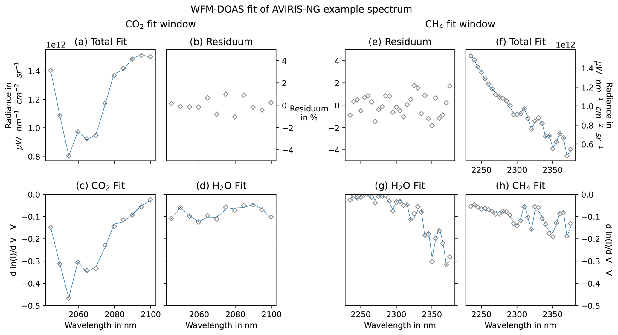
Figure 1Example fit result of the WFM-DOAS retrieval for AVIRIS-NG data. The left block (a–d) shows the CO2 fitting window (2040–2100 nm), and the right block (e–h) shows the CH4 fitting window (2235–2380 nm). In panels (a) and (h), the fit result is shown as a solid blue line, while the actual measured intensities are shown as gray diamonds. The difference between the gray diamonds and the line is the residuum which is shown in panels (b) and (e). In the second row, the scaled weighting functions for CO2 and H2O in the CO2 window (c, d) and for CH4 and H2O in the CH4 window (g, h) are shown as solid lines. The gray diamonds show the fit result plus the residuum to assess if the residual structures are larger than the actual fitted structures. In the CH4 fit window, the residuum shows some structure which might indicate some residual correlation between water vapor and methane signature in the real measurements which can not be fully resolved by the retrieval.
The WFM-DOAS retrieval produced profile scaling factors (PSFs) which scaled the weighting functions of CH4, CO2, H2O, and temperature in a linear fit. An example fit of AVIRIS-NG data with the resulting residual structures is shown in Fig. 1. The light passed the air mass above the aircraft once on the downward path to the Earth but transected the air mass below the aircraft on both downward and upward paths. Consequently, the retrieval was more sensitive to atmospheric changes below the aircraft than above. This was captured by the averaging kernel which represented the sensitivity of the instrument to changes at a specific altitude layer. In our case, strong local enhancements in atmospheric methane were confined below the aircraft, so we multiplied the total column enhancements by the inverse of the averaging kernel for the air mass underneath the aircraft (kAK) to determine the true enhancement of CH4 caused by an emission source near the ground.
We did not retrieve the pressure profile or scattering properties. This, and also other effects like surface elevation changes, could alter the light path and therefore the absorption strength which would be detected as an enhancement. We used the proxy method to correct the retrieved column enhancement for those effects (see also Frankenberg et al., 2005; Schneising et al., 2009; Krings et al., 2011). Specifically, we divided the derived scaling factor of CH4 by the scaling factor of another well-mixed gas which was assumed to be constant for the region of interest and time of overflight. For this work, we used CO2 as a proxy because of its spectral proximity to the CH4 absorption band, resulting in the proxy
Finally, we corrected the enhancements in a detected plume for large-scale effects by normalizing over the local background around the plume (PSFproxy, bg). The local column enhancement of CH4 below the aircraft in a plume (CH4,enh) was then
A discussion of the biases introduced by the assumptions made for the WFM-DOAS retrieval are studied in the sensitivity analysis in Sect. 3.3.
3.2 Comparison of major fitting windows in the SWIR spectral range
For the MAMAP instrument, the fitting window was ∼ 1630–1675 nm for CH4 and ∼ 1592–1617 nm for CO2 at 0.9 nm spectral resolution due to the sensor design (see Krings et al., 2011; Gerilowski et al., 2011). AVIRIS-NG additionally offered the possibility to fit the CH4 and CO2 absorption lines between 2000 and 2400 nm for the retrieval of CH4, although at a coarser spectral resolution of 5.5–6.0 nm. For example, the IMAP-DOAS retrieval successfully retrieved CH4 concentrations from AVIRIS-NG data using the spectral regions of 2215–2410 nm for CH4 and 1904–2099 nm for CO2 (Thorpe et al., 2017).

Figure 2The high-resolution simulated spectra (in panels a and b green) are convolved with the slit function of AVIRIS-NG and sampled to the AVIRIS-NG wavelength grid (solid black line in panels a and b). Panels (c) and (d) show the weighting functions, i.e., the change in intensity due to a change in atmospheric concentration for CH4 (blue), CO2 (black), and H2O (red). The shaded areas denote the fitting windows for CO2 (gray) and CH4 (light orange).
For a first assessment of those absorption bands, we convolved a simulated high-resolution spectrum and the corresponding weighting functions for CH4, CO2, and H2O with the AVIRIS-NG instrument spectral response function. We used a Gaussian spectral response for which the full width at half maximum (FWHM) values were distributed as part of the data set. Figure 2 shows the results of convolution and resampling to the AVIRIS-NG wavelength grid.
Both fitting windows had their advantages and disadvantages, especially for the lower spectral resolution of AVIRIS-NG. Around 2300 nm, the absorption features of CH4 were about a factor of 2 stronger and had a more pronounced structure which could lead to a better detection of methane changes. Around 1650 nm, the at-sensor radiance was nearly twice as high for the same albedo, which could mean a higher signal-to-noise ratio. Additionally, there was less overlap with water vapor absorption features near 1600 nm.
We used a two-step approach to find the best fitting window: first, we created a spatially averaged spectrum over a homogeneous surface elevation and surface type to reduce the instrument noise and systematic influences; then, we optimized the edges of both fit windows for fitting the gas features in each window. As a measure of fit quality, the root mean square error (RMSE) between measurement and fit result was used. For CH4, the best fitting windows were 1625–1700 and 2235–2380 nm and for CO2 1550–1620 and 2040–2100 nm (see also Fig. 2). For simplicity, the fitting windows between 1550 and 1700 nm will be called “weak windows”, and the fitting windows between 2040 and 2380 nm will be called “strong windows” in the following parts according to the depth of the absorption features.
To assess the measurement precision in each window, we selected a homogeneous, flat, bright area which contained no potential sources. We then applied the retrieval to the whole flight line containing this test case for each of the fitting windows and gases. These initial results showed detector-column-dependent stripes (see Sect. B in the Appendix). To correct this effect, we normalized the , , and for each pixel by the median PSF of its corresponding detector column. We selected the median for resilience against outliers which could otherwise have a large impact on the correction
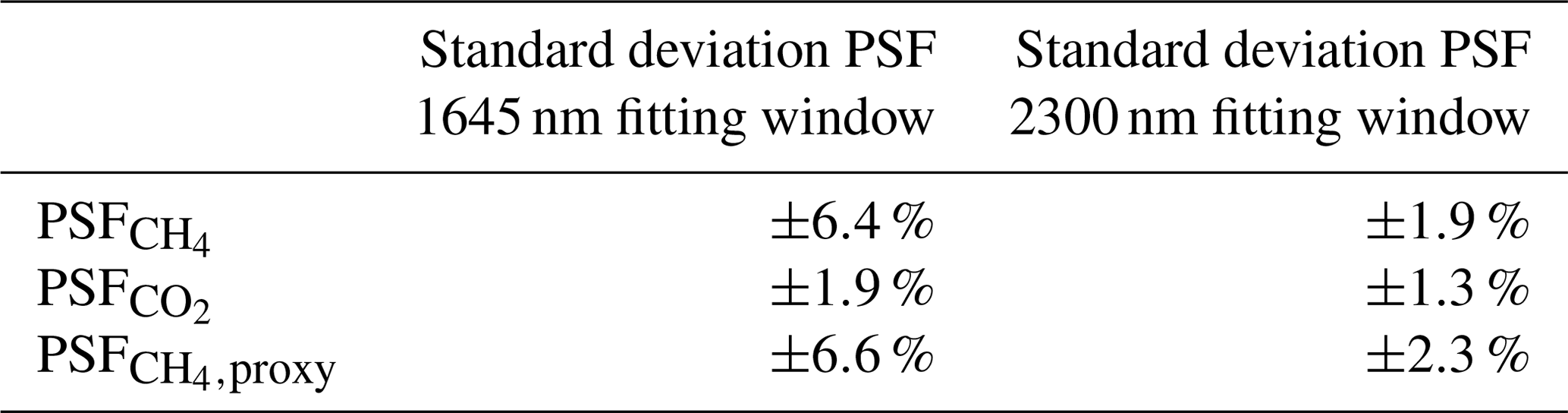
After destriping, we compared the standard deviation in the test case region of the weak and strong window retrieval results of , , and (Table 1). The retrieved and were noisier in the weak window by a factor of 3.3 and 2.9, respectively. The retrieved was noisier by a factor of 1.5 in the weak window. Therefore, we only used the strong windows in later analyses.
Table 1Comparison of the standard deviation of , , and in the two fitting windows around 1645 and 2300 nm for the AVIRIS-NG FWHM (≈6 nm). The standard deviation was calculated over a homogeneous and flat area with no visible plume and possible source inside. The statistical uncertainties in and are therefore uncorrelated.
3.3 Sensitivity analysis
In addition to the noise in the spectra, uncertainties and variability in the assumed constant atmospheric background parameters could lead to errors in the retrieval results. To assess the magnitude and influence of these deviations, we performed multiple sensitivity analyses. We used a common set of geometric and atmospheric parameters to model the background spectrum. We then perturbed these atmospheric parameters to create synthetic AVIRIS-NG observations at instrument spectral resolution. Next, we applied the WFM-DOAS algorithm to these simulated measurements and assessed the systematic offset from the expected PSF value for , , and . To assess the influence of linearization on the retrieval results, we did not include instrument noise in this analysis. The background simulation was based on the parameters extracted for one flight line observed with a nadir viewing angle. The CH4 enhancements and a plume from this flight line are shown in Fig. 8.
Table 2Parameters studied in the sensitivity analysis and the range in which deviations were analyzed. The second column shows the background scenario used as “truth” in the sensitivity study. The third column notes the range of the perturbation of the parameters. Parameters not mentioned here were constant and estimated as described in Sect. 3.1 for the flight line ang20170811t192639.
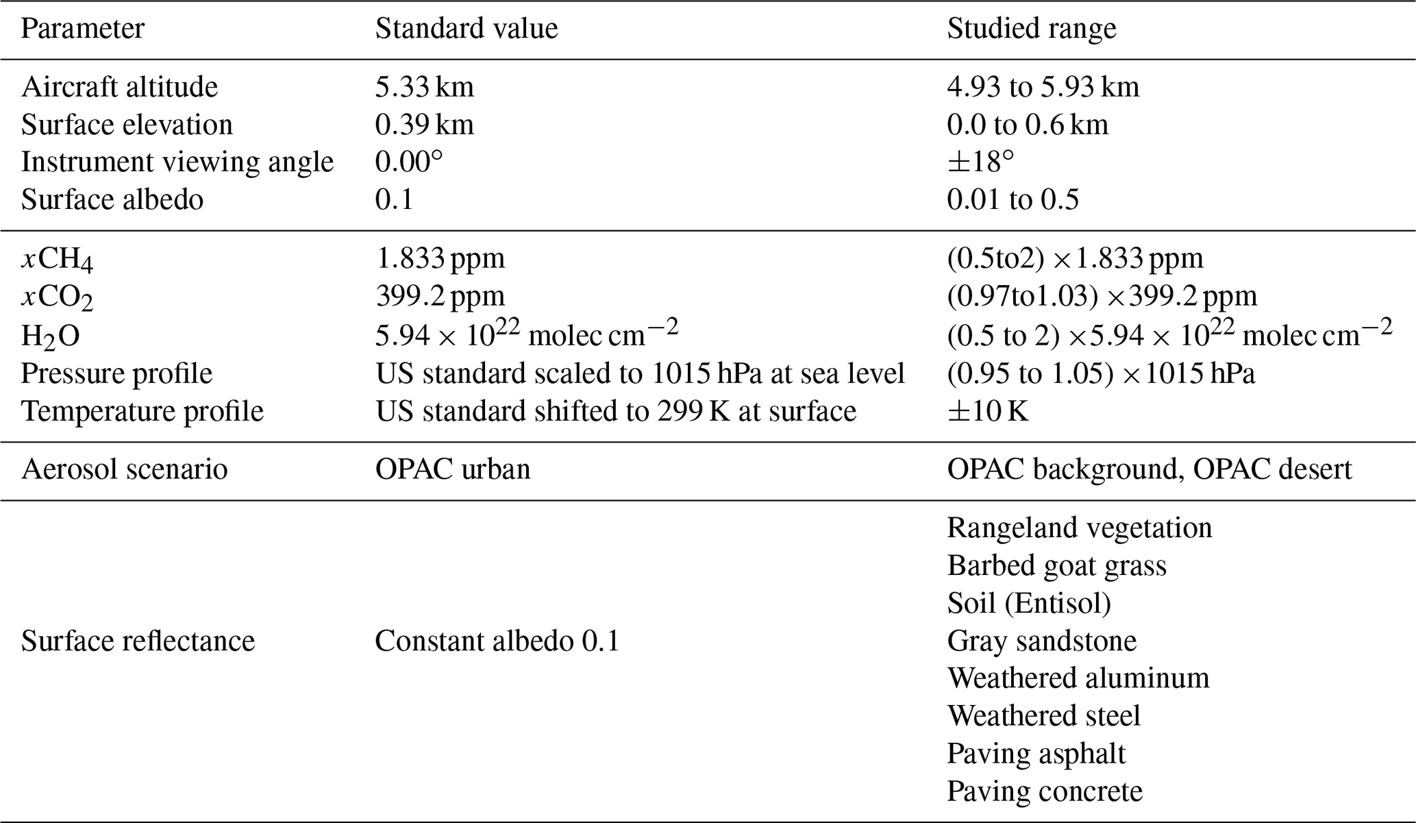
For the sensitivity analysis, we perturbed the following set of parameters (Table 2): the aircraft altitude, the surface elevation, the instrument viewing angle (i.e., the instrument zenith angle), and the surface albedo as geometric parameters, as well as the total columns of CH4, CO2, and H2O and the pressure and temperature profiles as atmospheric parameters. Additionally, we used selected spectral reflectance spectra of different surfaces instead of a spectrally uniform albedo and examined two additional aerosol scenarios. We did not analyze the sensitivity to the solar zenith and azimuth angles since these angles were effectively constant over the time span of a flight line. In addition, we did not analyze the instrument azimuth angle dependency since the flight tracks were nearly straight and the azimuth angle was therefore effectively constant for a flight line. Finally, we did not evaluate sensitivity to the spectral response function and wavelength calibration since these were adjusted during conversion of the raw digital numbers to radiometric data cubes (Chapman et al., 2019).
The viewing angle variations were chosen to represent the range of the AVIRIS-NG viewing angles. The surface elevation and aircraft altitude deviation were chosen to represent plausible deviations over one flight line. Temperature deviations were chosen to be relatively large as the temperature profile at the time of overflight for the specific ground scene might deviate quite a lot from the ERA-5 reanalysis due to the spatial and temporal resolution of the model output. The pressure scaling was chosen to represent a possible range of deviations, erring in favor of a conservatively high deviation for the observed scales. The albedo deviations covered the range which was expected around 2100–2300 nm (Chen et al., 2006).
The scaling of the CO2 column and the H2O column spanned the natural deviations in CO2 and water vapor from the assumed background to establish an upper bound on errors from these effects. The range for the total column of CH4 covered the range which might be observed directly over or near a strong source. However, in most ground scenes containing a plume signal, the enhancement was well below 20 % and for smaller plumes normally even near the source well below 10 %.
The reflectance spectra in the sensitivity analysis included surfaces present in the survey region or associated with oil and gas infrastructure. The spectral reflectances were based on the ECOSTRESS Spectral Library (Meerdink et al., 2019; Baldridge et al., 2009) and on the US Geological Survey Spectral Library, Version 7 (Kokaly et al., 2017). They contained spectra from a surface covered by a typical plant of the Canadian savanna, sandstone, sand, and rangeland surfaces and anthropogenic structures such as aluminum, steel, and paving substances. The reflectance spectra are shown in Fig. 3.

Figure 3In panel (a), the weighting function for CH4 is displayed. In panel (b), the reflectance spectra covered in the sensitivity analysis are shown. Especially for the paving concrete, one can see a similar broadband shape compared to the weighting function of CH4, which is caused by calcium carbonate (limestone).
The background aerosol scenario was assumed to be an optical property of aerosols and clouds (OPAC) (Hess et al., 1998) urban aerosol scenario (same as used in Krings et al., 2011) as we were interested in emissions from anthropogenic infrastructure. To determine the magnitude of influence of the aerosol scenario on the retrieval, we used additionally simulated measurements with an OPAC background and desert aerosol scenario.

Figure 4Sensitivity analysis of WFM-DOAS to the examined input parameters of the SCIATRAN radiative transfer calculation. The absolute deviation between the retrieved and the expected (blue), (orange), and (green) is plotted for each parameter. With the proxy method, the deviations are reduced for all parameters except for scaling in the total columns. For deviations in CO2, the proxy is worse than the single CH4 retrieval (see also Sect. 3.3).
After retrieving the profile scaling factors of CH4 and CO2 for each simulation, we calculated their deviation from the ground truth defined in the simulations. We also calculated the deviations for the CH4 proxy method described in Sect. 3.1 and plotted the errors as a function of the perturbation of each parameter in Fig. 4. While the observed uncertainties in the single profile scaling factors were quite high (orange and blue curves), for example, up to 10 % for an elevation change of approximately 400 m, they were highly reduced by the proxy method (green curve). The influence of the surface spectral reflectance is shown in Table 3 and discussed at the end of the section.
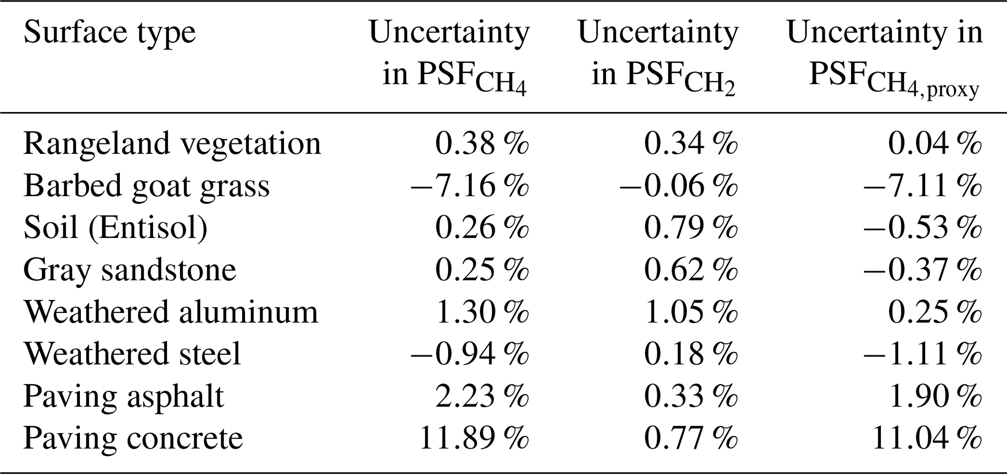
Table 3Uncertainty estimate of , , and due to the assumption of a constant albedo over different surfaces. As long as there is a constant surface type, a large value does not principally hinder source detection. However, especially paving or man-made structures vary spatially with non-man-made structures, so false positive hits due to surface reflectance are possible.
For aircraft altitude, temperature shifts, surface pressure scaling, and viewing angle of the instrument, the maximum deviation from the ground truth for remained well below 0.5 %. Also, for most albedo values, the maximum deviation remained below 0.5 %. For a very low albedo of 0.01, results of the single retrievals and the proxy method both degraded considerably. We examine low radiance ground scenes further in Sect. 3.4. For large perturbations of the surface elevation of 400 m, the proxy method reduced the error only to around ±3.6 %. The different aerosol scenarios did not introduce major errors either. For the OPAC background scenario, the error was well below 0.1 %, and even for the OPAC desert aerosol load, only an error of −0.2 % was introduced.
For perturbations of CH4 and H2O, errors between the true and retrieved PSF grew the larger the perturbations got. WFM-DOAS assumes a linear relationship between gas enhancement and radiance, but this assumption does not hold for large deviations from the background. This will also occur for CO2 when choosing larger deviations from the background.
When we perturbed CO2, the application of the proxy method increased the error in methane. When only CO2 was varied, the methane column alone was retrieved correctly in the standard retrieval. Similarly, the retrieval correctly estimated the total column of CO2. However, in the proxy method the retrieved was divided by the retrieved so that a decrease in CO2 led to an apparent increase in CH4 and vice versa. This meant that CO2 emission sources could mask CH4 emissions if the relative single column enhancement of CO2 is similar or greater than that of CH4. As the retrieval noise is similar for both gases (Table 1), this would be visible as a CO2 point source in the map.
For the scaling of CH4, the proxy method did not reduce the deviation in the retrieved enhancements from the true enhancements, as expected. However, the large deviations for strong enhancements (11 % underestimation for 100 % increase) would nevertheless mean a clearly detectable signal in the retrieved CH4 maps. Smaller deviations (±20 %) from the background profile would induce only small (<1 %) underestimations. Consequently, for inversions of large emitters, the emission might be underestimated near the source where the large enhancements are located. In cases with large concentrations near the source, emission estimates should only be performed further down the plume.
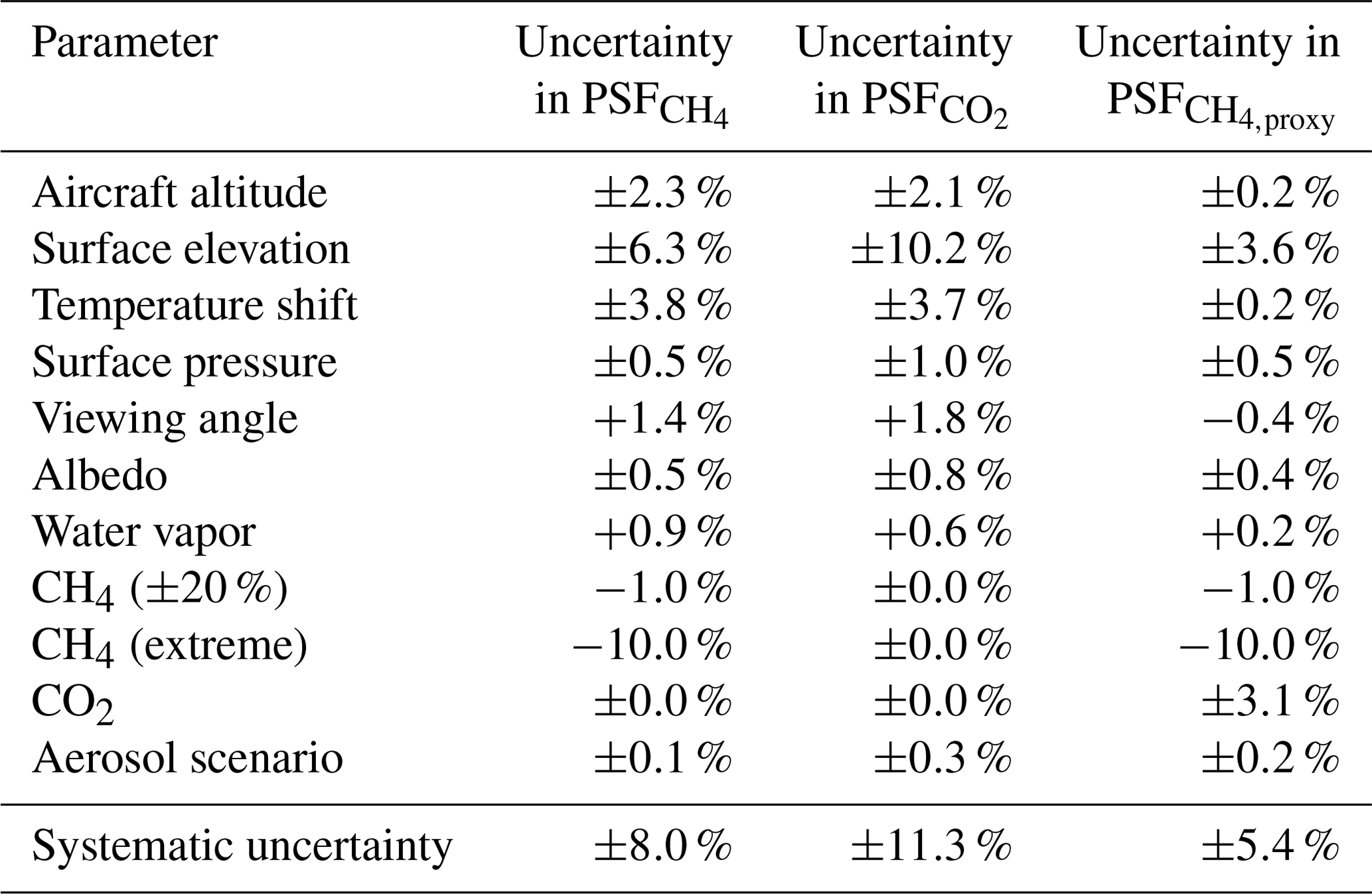
To estimate the total systematic uncertainty, we combined all uncertainties in Table 4 aside from the extreme CH4 case in quadrature. This led to maximum systematic uncertainties of ±8.0 % for , ±11.3 % for , and ±5.4 % for due to the simplification of the radiative transfer calculation to one single background spectrum and set of weighting functions. This uncertainty defined the large-scale deviations possible in one flight track and should not be confused with the single pixel precision of the column enhancement, nor did that automatically limit detection. As parameters such as surface elevation in normal cases only vary smoothly, a plume signal on top of this bias is still detectable. However, a problem may occur if large amounts of CO2 are co-emitted with a weak methane source. In this case, there could be a (partial) masking of the plume due to the negative bias introduced by CO2.
Table 4Uncertainty estimate resulting from the assumed constant atmospheric and geometric background parameters. For each parameter, the maximum deviations for and , as well as for , are listed. For albedo, the largest value was excluded from this table (see main text). For CH4, two different cases are regarded. The case CH4 (±20 %) is valid for most of the plumes and is relevant for detection of smaller sources. The extreme case (100 % increase) is only relevant near very strong sources and is excluded from the averaged systematic uncertainty. The absolutely correct retrieval of when changing CO2 is due to the relatively small range of change in CO2 investigated. However, this induces relatively large uncertainties in .
In contrast to those biases, the different surface types induce widely varying biases (Table 3) at AVIRIS-NG spectral resolution. The proxy method reduced these errors for some surfaces but not all. For rangeland vegetation, soil, gray sandstone, and weathered aluminum, the bias after application of the proxy was well below 1 %. However, for weathered steel and paving asphalt, the bias increased to 1 %–2 %, while for barbed goat grass and paving concrete (i.e., limestone), the bias due to the reflection properties was greater than 7 %. This meant that even after application of the proxy, some residual influence of the surface reflectance will remain. Paving concrete would be especially likely to cause a false positive since it induced a large positive bias. However, this would be highly correlated to structures visible in the RGB images of the scene. Barbed goat grass, on the other hand, led to a large underestimation of the total column. However, this surface type normally occurs over large patches of land so that local enhancements on top of this bias should be detectable in most cases.
3.4 Filtering of poor fits
With the estimate of the influence of the background assumptions in place, we performed radiative transfer calculations for the different flight tracks and applied the retrieval to the whole data set. Examining the data, it was obvious that the retrieval sometimes failed to retrieve meaningful results. Especially over surfaces with low spectral reflectance and therefore low signal on the detector, it produced mostly noise with profile scaling factors ranging from below 0 to largely over 2 and dramatic changes between neighboring ground scenes (see Fig. 5). This effect, due to the low SNR over dark surfaces, indicated the need to filter out low-radiance ground scenes. For IMAP-DOAS, Ayasse et al. (2018) concluded in a simulation study that at-sensor radiances below 0.1 µW cm−2 nm−1 sr−1 in the background signal led to significantly more inaccurate estimates of the methane column. In this study, we analyzed measured radiance spectra to estimate the radiance below which the retrieval results were not trustworthy.
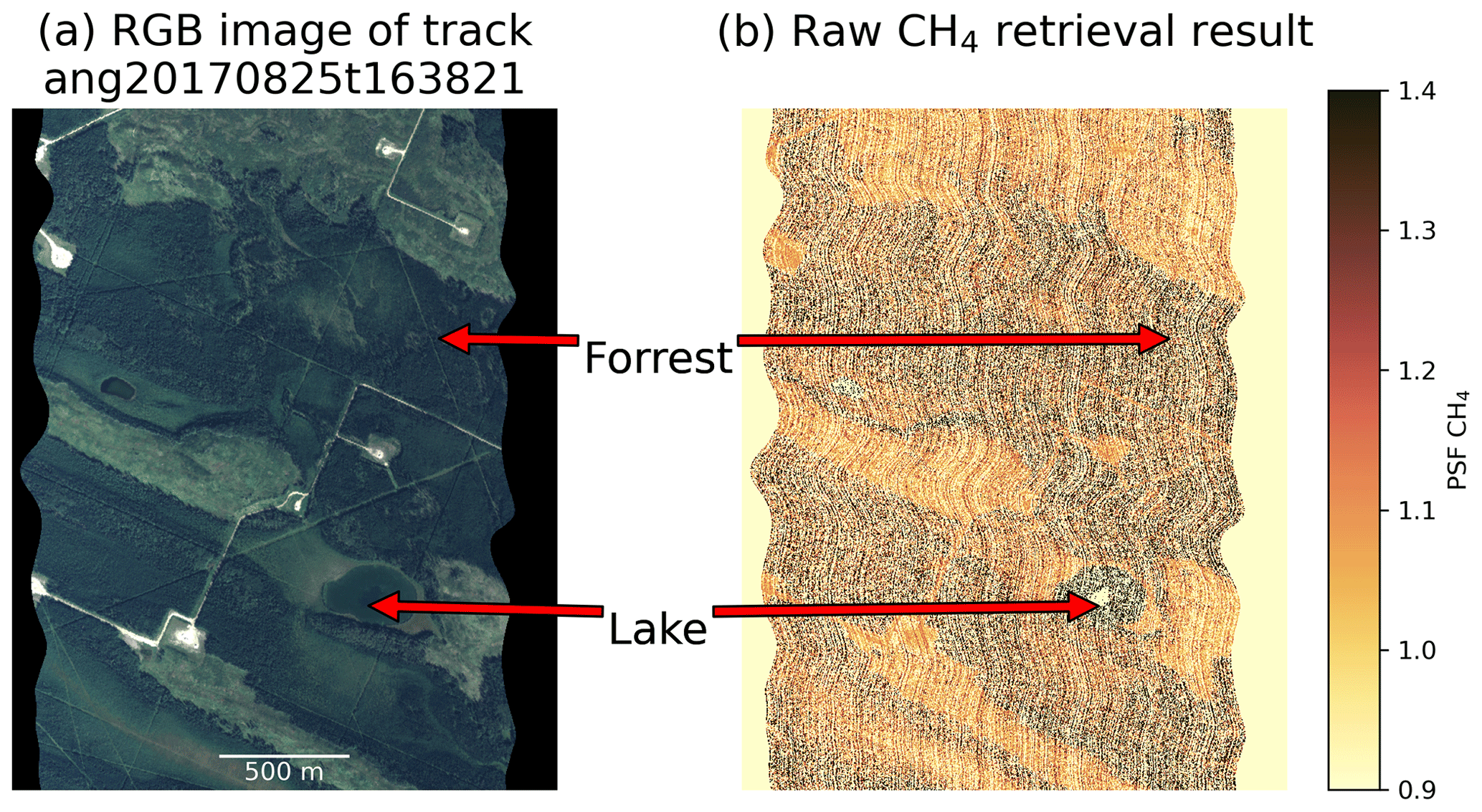
Figure 5Raw retrieval results of CH4 (pure , not filtered and destriped, no proxy method applied) over a scene with large forest areas and a lake as an example of a dark scene. The retrieval produced large noise over surfaces with low spectral reflectance like forests or lakes.
The threshold was determined by the following procedure. For each ground scene, the difference between the measured and the fitted spectra was calculated for each spectral pixel after the retrieval. These values were added in quadrature to get the root mean square difference between fit and measurement (RMS). This RMS value was then plotted over the radiance at 2140.0 nm in box plots with 0.05 µW cm−2 nm−1 sr−1 bins on the horizontal axis (Fig. 6) for the whole data set. For low radiances, this difference increased drastically, implying a strongly reduced fit quality. As a compromise between coverage and quality, we introduced a threshold of 0.1 µW cm−2 nm−1 sr−1. The filter rejected all retrieval results for which the radiances at 2140.0 nm were below this value. We also rejected measurements with an RMS over 2 % to remove the worst outliers. Interestingly, for very bright surfaces, the spread of the upper whisker, denoting the 75th to 95th percentiles, is increased. This could have been from surfaces such as paving materials or other anthropogenic structures, for which the reflected spectrum already had interfering features similar to the absorption of CH4 at the AVIRIS-NG spectral resolution (see also Sect. 3.3 and Table 3). These results agree with the findings of Ayasse et al. (2018).
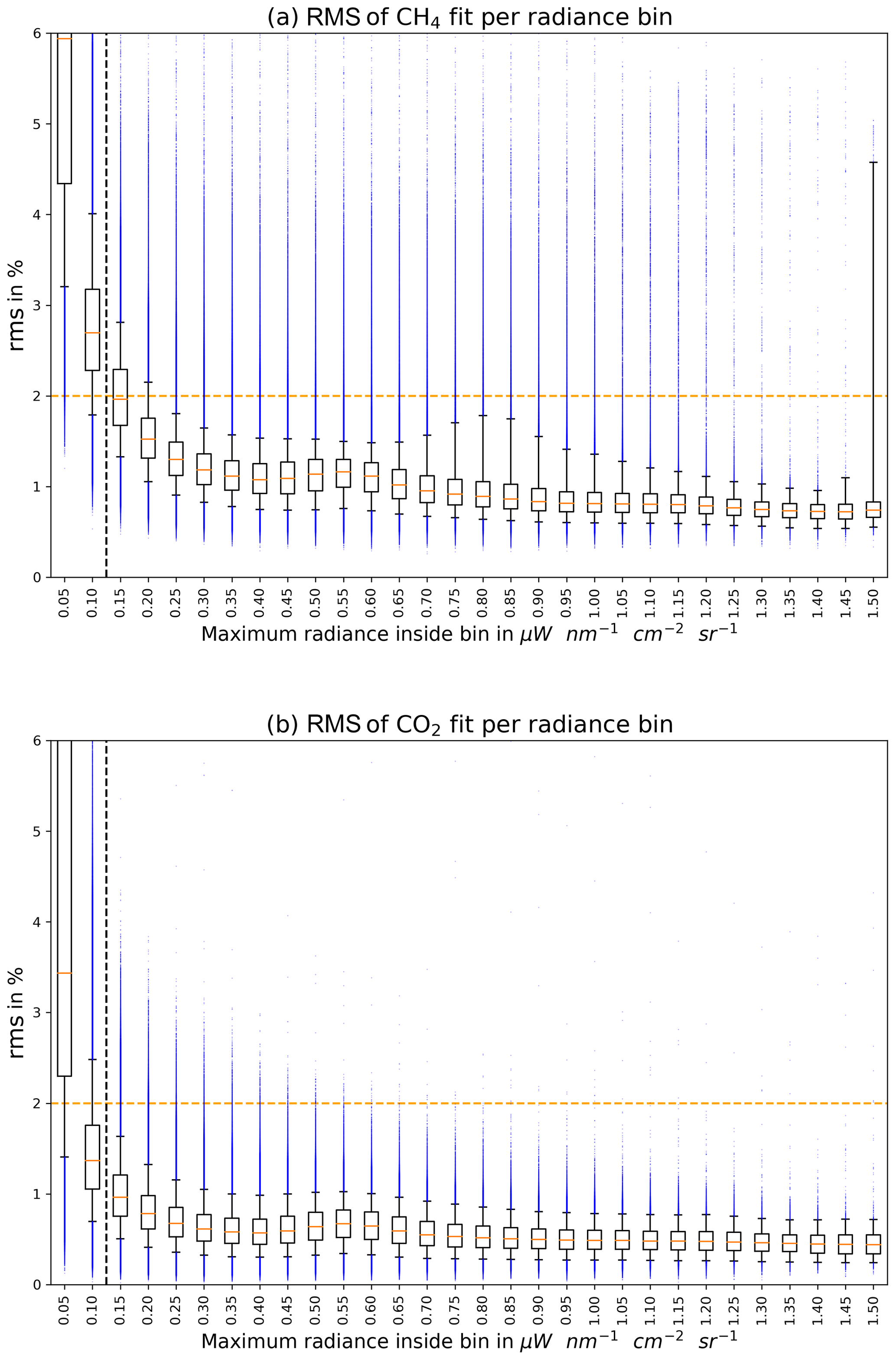
Figure 6Difference between fit and measurement (RMS) over radiance at 2140.0 nm. The box indicates the first to third quartile range, the whiskers denote the 5th to 95th percentiles, and the small orange line inside the box is the median RMS value of the according radiance bin. The small blue dots denote outliers outside the 95th percentile. For low radiances, the fitting quality decreases significantly. Therefore, all measurements over surfaces with radiances below 0.1 µW cm−2 nm−1 sr−1 are filtered out (dashed black vertical line). Results with RMS higher than 2 % are filtered out as an additional quality flag (dashed orange line).
4.1 Detection of plumes
For the detection of plumes, we filtered the retrieved CH4 values (Sect. 3.4), removed striping (Sects. 3.2 and B in the Appendix), and calculated the final CH4,enh according to Eq. (2). The proxy method proved necessary, otherwise diffuse CH4 enhancements would have been mistaken for true enhancements due to emissions of CH4. This can be seen in Fig. 7, in which diffuse enhancements in the pure CH4 results vanished completely after applying the proxy method.
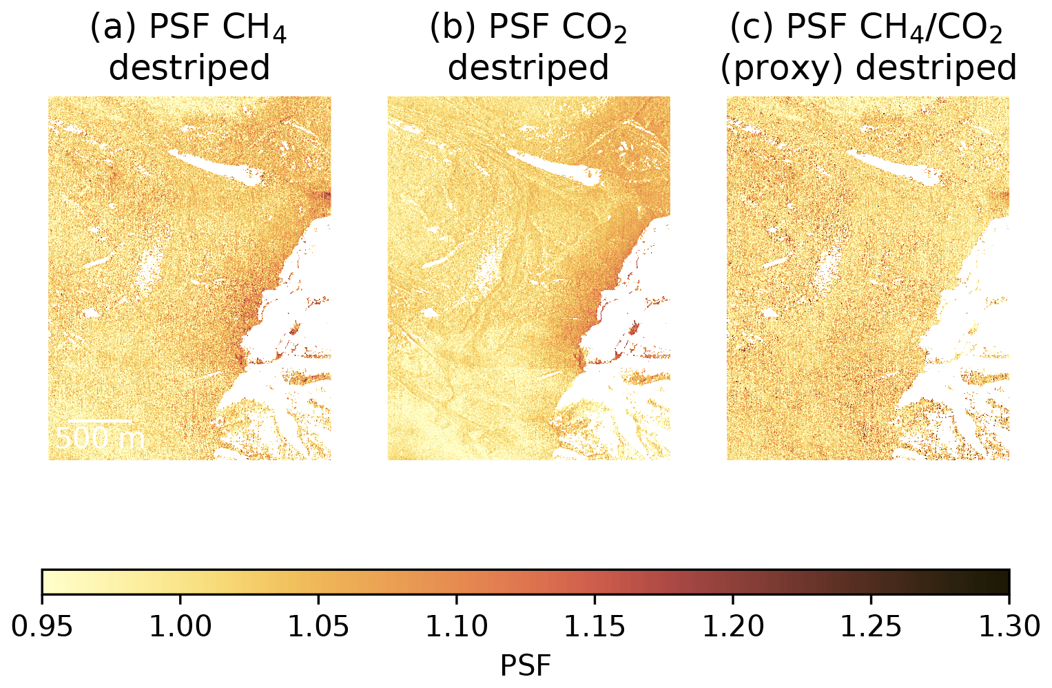
Figure 7Example of the effect and necessity of the proxy method from flight line ang20170823t180156. In panel (a), the destriped is shown. Simply analyzing this image, one could assume a diffuse enhancement due to perhaps coal mining activities as this is part of an open-cast coal mine. In panel (b), the destriped is shown. There, a similar enhancement is visible. In panel (c), the destriped proxy results are shown in which this diffuse enhancement vanishes.
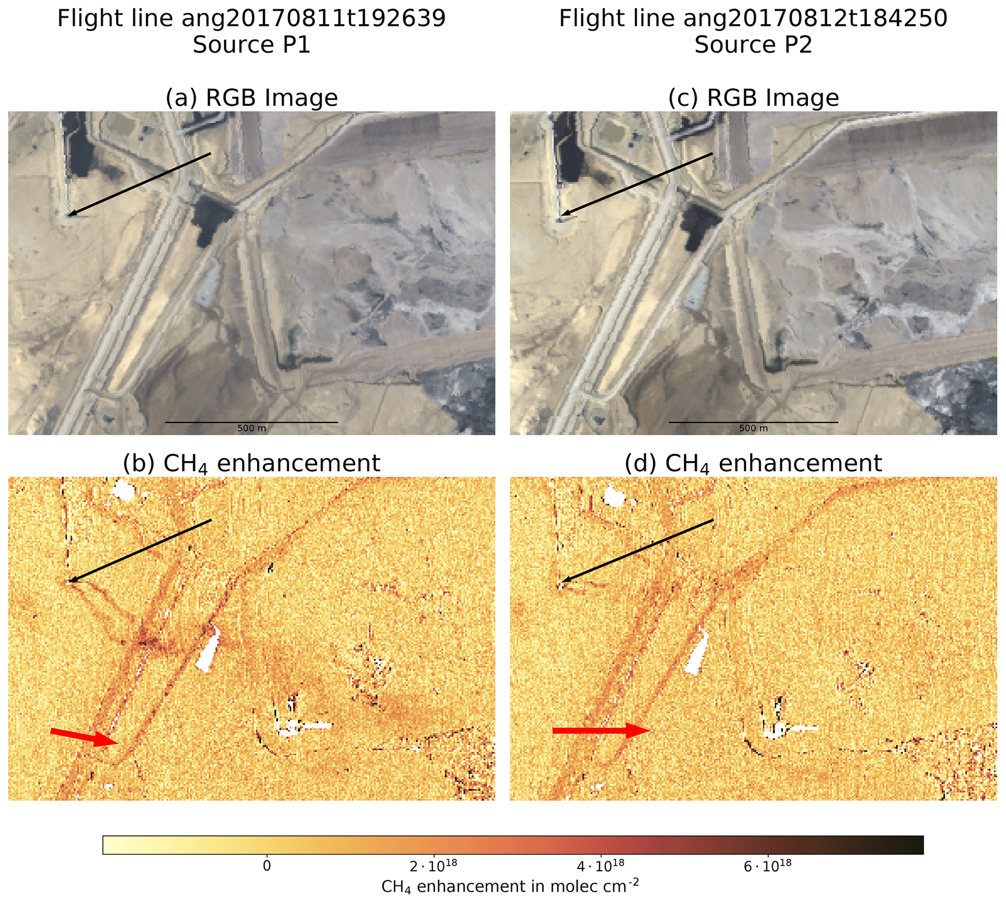
Figure 8Plume resulting from a cold vent. The black arrow denotes the source position, while the red arrow indicates the wind direction and wind speed according to ERA-5 data for comparison to the plume direction. In panel (d), the plume is much fainter most likely due to the higher wind speed. Especially in panel (b), a double plume structure is visible in the first part of the plume. As vertical and horizontal mixing takes place the further the emissions travel, the light passes through the plume twice, and the double plume structure vanishes. The roads are prominently visible in the retrieval results. It might be that this road is made of concrete or otherwise contains limestone.
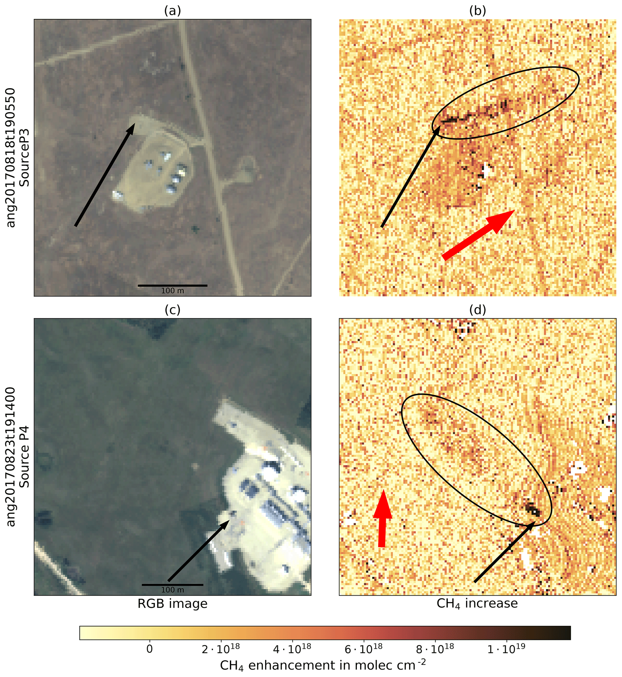
Figure 9Two additional plumes detected in the retrieval results, emanating from well pads. On the left (a, c), the RGB images obtained from radiances of AVIRIS-NG are shown. On the right (b, d), the according retrieval results are presented. The ellipse highlights the plumes. Additionally, the black arrows point to the source of the plumes, while the red arrow indicates the wind direction and wind speed according to ERA-5 data for comparison with the plume direction. The sources are located near grassland.
The final CH4,enh were plotted as images and were manually inspected for methane plumes. For the reduced data set used in this study (13 tracks), this approach detected several plumes in 10 out of the 13 tracks. However, many plumes were faint or located near infrastructure, making unambiguous detection difficult, or the plumes were very short. Therefore, we show plumes which extend over longer ranges and have unambiguous morphology in Figs. 8 and 9. The additional CH4 plumes and enhancements can be found in the Appendix in Sect. C. Those comprise, among others, emissions most likely resulting from open-cast coal mining (Fig. C1) or a well pad located in a forest (Fig. C2).
In Fig. 8, two overpasses of the same source on two different days are shown. On the first day (Fig. 8b), the plume structure was recognizable over a relatively long distance, while on the second day (Fig. 8d), the plume was only faintly visible in the vicinity of the source. This was most likely due to the wind speed which was significantly higher on the second day (7.6 m s−1) compared to the first day (3.7 m s−1). Assuming a constant emission, a wind speed higher by a factor of roughly 2 means a decrease in the column enhancements by a factor of roughly 2, which would significantly reduce the visibility of the plume in the retrieval results by diluting larger parts of the plume faster below the background noise.
In Fig. 8, a new interesting feature was observable at the source. There, we observed a double plume structure that was especially prominent during the first overpass. A comparison with the RGB image revealed that one part seemed to originate from the vent, while the other part seemed to originate from the top of the shadow of the vent. The vent released the plume several meters above the surface. Because the plume was very narrow near the source, the sunlight only passed the plume either before or after hitting the ground. As those two light paths were attributed to different ground scenes, the absorption and therefore the apparent CH4 enhancements were visible at two locations leading to the double plume structure. Further down the plume, atmospheric mixing took place, and the plume widened. Then, the sunlight passed through the plume both before and after hitting the ground, and the double plume structure vanished. A simple geometric consideration of the distance between the two plume structures (∼50 m), the solar and instrument zenith angles (∼42 and ∼2.5∘), and the vent height calculated from the shadow of the structure (∼55 m) and the solar zenith angle supported this hypothesis.
In Fig. 9, two plumes originating from well pads are shown. Both extended linearly from their source and were visible over approximately 100 m. While the first plume (Fig. 9b) originated from a cold vent (similar to Fig. 8), the emitting structure for the plume in Fig. 9d could not be identified from the RGB images. It seemed, however, that the source was located near the surface. This would also explain the large deviation in the plume direction from the wind direction acquired from the ERA-5 model data since the nearby forests could have significantly altered the wind direction near the surface.
Additionally, the plume detected over a coal mine ventilation shaft during the Four Corners measurement campaign in 2015 is shown in Fig. 10. The plume was nearly 1 km long with a straight profile except for a small diversion at the tip that suggested a change in wind direction.

4.2 Comparison of WFM-DOAS retrieval results with IMAP-DOAS and MF results
To assess the performance of the WFM-DOAS retrieval with respect to the IMAP-DOAS and MF retrieval results, a subset of the data was compared quantitatively. We focused here on the coal mine ventilation shaft plume for all three retrievals and additionally compared the WFM-DOAS results to MF results over plumes P1–P4. As IMAP-DOAS and the MF retrieve CH4 enhancements below the aircraft in parts per million times meters (ppm ⋅ m; ), we converted these retrieval results to enhancements in molecules per centimeter squared (molec cm−2; ) via the following equation:
where hairc is the distance between instrument and ground in nadir direction, and subcoltot is the number of dry molecules per square centimeter between aircraft and ground. The sub column below the aircraft was calculated on the basis of the profiles used for the WFM-DOAS retrieval.
Table 5Comparison of background noise of the retrievals based on the standard deviation of retrieval results near the plumes. As we only have IMAP-DOAS results for one plume, the other fields are left empty.
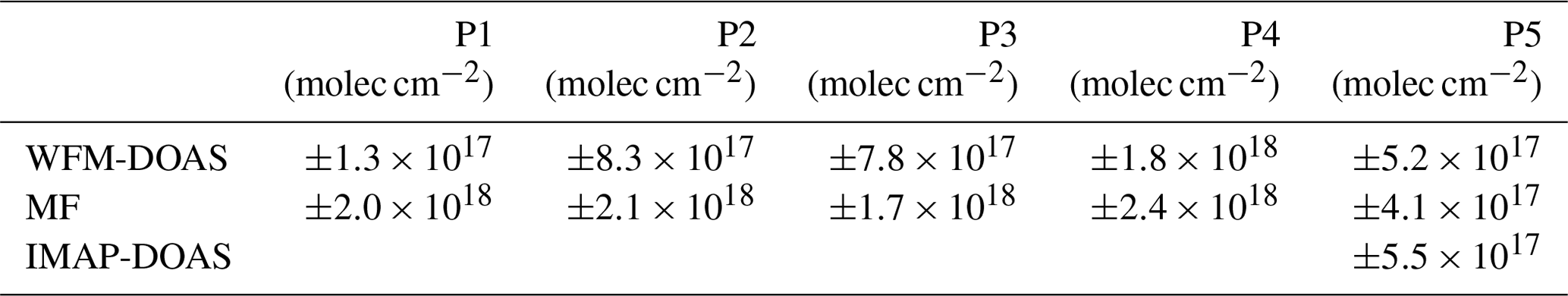
We compared the retrieval results in two different ways, focusing on retrieval scatter and retrieved enhancements. First, for the retrieval scatter, we calculated the standard error (1σ) of retrieved enhancements over areas near plumes P1–P5. This is summarized in Table 5. For all plume regions except P5, the retrieval scatter is lower for WFM-DOAS than for the MF results which indicate less retrieval noise. For P5, for which all three retrieval results were available, the background noise is very similar for all retrieval methods.
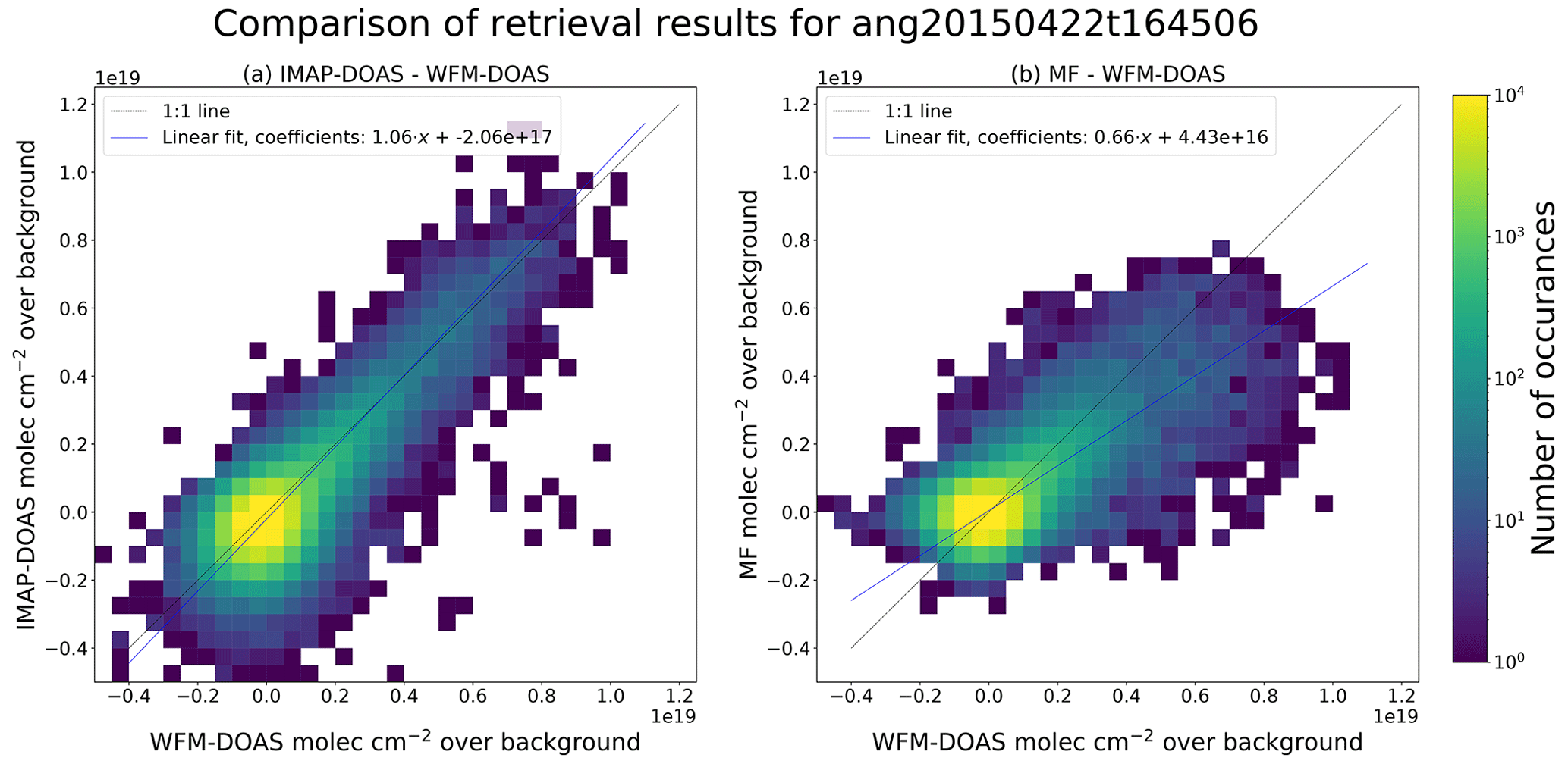
Figure 11Scatter plot comparison between IMAP-DOAS and WFM-DOAS (a) and MF and WFM-DOAS (b), respectively, for the coal mine ventilation shaft plume.
Second, to evaluate the agreement of the retrieval results, we additionally produced scatter plots of the central plume area. We added the 1 : 1 line and a linear fit to the scatter plots. For the coal mine ventilation shaft plume, all three retrievals agreed well in the retrieved enhancements, as can be seen in Fig. 11. Compared to the IMAP-DOAS retrieval, WFM-DOAS did retrieve slightly lower enhancements, while it did estimate slightly higher enhancements than MF.
Additionally, we compared the WFM-DOAS and MF results for plumes P1–P4 (see Fig. D1). For P3 especially, the higher enhancements located inside the plume agree well. However, for the other plumes, there is quite some mismatch between MF results and WFM-DOAS results. The cause for the disagreement is currently under investigation and might be related to the use of a standard gas target for the matched filter rather than calculating a target specifically parameterized for a given scene.
4.3 Flux and uncertainty estimation based on cross-sectional flux method
To estimate the fluxes for the selected sources, we applied the cross-sectional flux method (White et al., 1976). As this method is computationally and conceptually simple, it could well be used for initial estimations of source strengths. It had successfully been utilized for the estimation of emissions detected in remote sensing measurements (for example in Krings et al., 2011; Frankenberg et al., 2016; Krautwurst et al., 2017; Varon et al., 2019). In this method, one calculates the flux F in kilograms per hour through a transect orthogonal to the wind direction with length segments dxi in meters using the total column enhancements in molecules per square centimeter at position i along the transect:
The wind speed u in meters per second is assumed to be constant in time and space for the time of overflight. For the detected AVIRIS-NG plumes, this assumption was valid as these plumes had been sampled within seconds. The wind speed was extracted from nearby weather station data (see Sects. 2.2 and A), while the wind direction was visually estimated from the observed plume directions by drawing the best fitting line from the source along the plume. The factor s kg h−1 molec−1 converted the flux to kilograms per hour.
We defined the local background for CH4,enh for each cross section as the region outside of the plume on each side. Then, we calculated the PSFproxy,bg for the normalization to the local background using a linear fit between both local background regions. This background fit reduced slight gradients present in the background concentration to accurately estimate the column enhancements originating from the source.
As is observable in Figs. 8 and 10, there were gaps and accumulations along the plume. These were caused by eddies and short gusts which disrupted the plume structure. To account for that atmospheric variability, we defined multiple cross sections along the plume, each one pixel apart. We then calculated the flux for each of the cross sections. The final flux estimate was the mean value of the single fluxes through all cross sections.
For the plumes shown in Fig. 8 (in the following P1 and P2 for panels b and d, respectively), Fig. 9 (P3 and P4 for panels b and d, respectively) and Fig. 10 (P5), the methane flux was calculated using the cross-sectional flux method. We selected plumes P1 and P2 for two reasons: P1 was visible for approximately 200 m before crossing the road, making it possible to define multiple cross sections through the plume and thus leading to a strong reduction in the uncertainties. This was the only source observed twice in an emitting state by AVIRIS-NG, which allowed for the comparison of the flux estimates for two overflight times. It originated from a vent in a bitumen extraction site. P3 and P4 shown in Fig. 9b and d also showed a well-shaped straight plume which was favorable for the cross-sectional flux method. In Figs. 8b and 9b, a clear bias due to the underlying road surface was visible. In both cases, cross tracks that overlapped with this bias were excluded from the flux estimation. P5 showed the strongest enhancements over the longest range, which allowed us to calculate the flux through over 100 different cross tracks through the plume which greatly reduced the uncertainty due to atmospheric variability.
Application of the cross-sectional flux method on all plumes yielded the following emission estimates. For P1, a mean flux of (196±94) kg h−1 was calculated, while for P2, the mean flux was (155±71) kg h−1. For P3 and P4, the mean fluxes were (157±109) and (204±116) kg h−1, respectively. For P5, the mean flux was (1220±450) kg h−1. The wind speeds for the different plumes according to the weather stations were 3.7, 7.6, 3.9, 4.2, and 4.1 m s−1 for P1–P5, respectively.
We estimated the uncertainty in the flux via Gaussian error propagation from the standard error of the single components of Eqs. (4) and (2) while additionally accounting for the atmospheric variability. The contribution and derivation of the main error sources for P1 is shown below. We used the same procedure to estimate the uncertainty in the other sources.
We estimated the single pixel precision for each plume region by analyzing the local background of the plume. We used the 1σ standard deviation of the local background as measure of the retrieval noise and included the uncertainty due to small variations in CO2 which might have been co-emitted from the flare or collocated to the plume but which were below the noise of the pure . This led to a single pixel precision of ∼3 % of the CH4 background column which translated to an uncertainty in the final flux of ±36 kg h−1.
The uncertainty due to atmospheric stability was calculated as the confidence interval of the fluxes through all cross sections. This amounted to an uncertainty in the final flux of ±33 kg h−1.
For the wind, we assumed an uncertainty of ±1.5 m s−1 according to the 1σ standard deviation of the hourly wind measurements of ERA5 compared to inland measurement stations (Minola et al., 2020) to account for the partly larger distance between weather stations and plume locations, as well as the usage of hourly mean data from the weather stations. As the wind speed directly influenced the flux, and the uncertainty could not be reduced by simply taking more cross sections into account, this directly propagated to an uncertainty in the final flux of ±79 kg h−1.
The estimate of the background column was dependent on a scaled climatology. We assumed a ±5 % deviation as an upper limit of the uncertainty in the total column of CH4 around the plume compared to this climatology. This led to an uncertainty in the final flux of ±10 kg h−1, which was very small compared to the other uncertainties.
Table 6Inversion results and uncertainty estimate using the cross-sectional flux method for P1 and P2 (two overpasses of the same source on 2 consecutive days), P3, P4, and P5. The single pixel precision was calculated from the 1σ standard deviation of a background region for each plume. The atmospheric variability resulted from the confidence interval of the multiple cross-sectional fluxes. The wind uncertainty and total column uncertainty was assumed to be ±1.5 m s−1 and 5 %, respectively (see also text for explanation). For all inversions, the wind speed uncertainty is a very large uncertainty. While additionally for P2, the atmospheric variability induces similar large errors, for P3 and P4 this is much less the case. However, there the different surfaces lead to a much larger single pixel uncertainty. For P5, the error is dominated by the wind speed uncertainty.
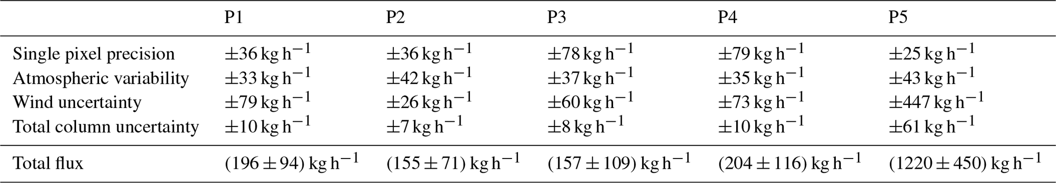
Assuming that those sources of uncertainty were uncorrelated, we combined them in quadrature. This resulted in an uncertainty in P1 of ±94 kg h−1. An overview over the contribution of the single error sources for all sources is given in Table 6. We emphasize that for all of these cases, the fluxes were calculated from snapshots and were only valid for the time of overflight.
Our estimates for P1 and P2 overlapped within their respective uncertainties, suggesting that the source may have been approximately constant on 2 consecutive days. The difference in the mean estimate could be explained by uncertainties in our assumptions of the wind speed and the stronger dilution of the plume on the second day (Fig. 8). For P2, additionally the wind speed uncertainty might be even higher as in such strong wind situations stronger wind gusts could also momentarily dilute the plume.
The WFM-DOAS retrieval provided an efficient and accurate way to handle AVIRIS-NG data quantitatively. In contrast to the IMAP-DOAS retrieval (Frankenberg et al., 2005; Thorpe et al., 2014), the WFM-DOAS retrieval is a non-iterative retrieval with precalculated radiative transfer calculations. This reduced the computational time needed for the retrieval while still delivering reliable local total column enhancements. On the other hand, the modeled background spectrum is adapted to the physical properties of the scene by scaling the trace gas columns and adapting the geometric parameters necessary to model the average light path over the scene in contrast to the more statistical approach used in the matched filter (Thompson et al., 2015). For most scenes, WFM-DOAS results showed less background noise than the MF results apart from the coal mine ventilation shaft plume.
The WFM-DOAS retrieval of CH4 in the two SWIR fit windows of AVIRIS-NG data produced much larger noise in the results for the weak window than for the strong window. The significantly less noisy WFM-DOAS results around 2300 nm most likely originated from the higher number of spectral data points for the fit and the stronger absorption features. Even though there was approximately half the amount of light reaching the detector at these wavelengths which reduced the SNR on the detector, the SNR was still high enough for a good retrieval.
Problems, however, arose over very dark surfaces or surfaces with reflection properties similar to absorption features of CH4 at the spectral resolution of AVIRIS-NG. This led to residual structures in the retrieved CH4 maps. Especially paved roads or other anthropogenic structures were observable. Even though the CH4-over-CO2 proxy method reduced false positives in many cases, there was still a remaining dependency of the CH4 results from the surface spectral reflectance for some surfaces like concrete or barbed goat grass. Additionally, the noise in the retrieval results varied over different surfaces which is reflected in the uncertainties in the flux inversions for the plumes.
Those effects could be mitigated by deploying and utilizing an imaging spectrometer specifically designed for the task of monitoring CH4 and CO2 concentrations such as the proposed Airborne Methane Plume Spectrometer (AMPS; Thorpe et al., 2016b) or the MAMAP 2D system currently being developed and built at the University of Bremen, Germany. Due to the higher spectral resolution, those instruments will have a higher sensitivity to smaller enhancements and should be less influenced by the surface reflectance properties, as is already the case for the MAMAP instrument (see, e.g., Krings et al., 2011).
A large uncertainty in the flux inversion of emission sources which can not be solved by advancing the imaging remote sensing instrument's characteristics arises from the wind speed estimation. Additional measures have to be taken to reduce this uncertainty. For example, in situ wind measurements in the boundary layer at the plume location could additionally be made (see, e.g., Krautwurst et al., 2017; Krings et al., 2018). This approach is especially useful when airborne in situ measurements are included in the campaign design. Another possibility includes the deployment of wind lidars (Wildmann et al., 2020), which is similar to the approach taken in the Carbon Dioxide and Methane Mission (CoMet). However, for large surveys or transects, this is not feasible anymore, especially when the source locations of the plumes are not known prior to the flights. There, either advancing to local wind models with much higher spatial resolution such as the GRAL model (Berchet et al., 2017) or the MECO(n) model (Kerkweg and Jöckel, 2012) could lead to a significant uncertainty reduction, but those models have to be carefully validated. Also, methods such as the integrated mass estimation (IME; Jongaramrungruang et al., 2019), which uses empirically derived correlations between surface wind, flux rates, plume shape, and mass enhancement in the plume to estimate the wind speed and the flux, could help in estimating the emissions independent from local wind models or wind measurements. Additionally, more sensitive remote sensing instruments could observe the plume over longer distances, where the plume is likely better mixed in the boundary layer and the horizontal extent of the plume is less influenced by turbulence and gusts so that the modeled wind speed in the boundary layer likely better matches the wind speed inside the plume.
We successfully adapted and applied the WFM-DOAS retrieval to AVIRIS-NG data and estimated the uncertainties in this method. In the data set, we were able to detect several point sources. An estimation of the methane emissions of a vent revealed emissions of (196±94) and (155±71) kg h−1 on 2 consecutive days, while two other sources related to gas extraction emitted (157±109) and (204±116) kg h−1. The emission of the coal mine ventilation shaft was estimated to be (1220±450) kg h−1. These source strengths are quite common, as indicated by the log normal distribution of sources in the Four Corners region (Frankenberg et al., 2016). A large source of uncertainty in the flux inversion was the wind speed estimate as no collocated wind speed measurements near the surface were collected. Also the atmospheric variability played an important role for shorter (i.e., smaller) plumes. This influence is reduced for longer plumes, as more tracks are available for the flux estimation. The noise in the retrieval results varied with different surfaces, which contributed notably to the uncertainty in the flux estimate. For the high wind situation, parts of the plume might have been additionally missed due to the higher dilution.
The comparison between IMAP-DOAS/MF and WFM-DOAS resulted in good agreement for the coal mine ventilation shaft and P3. However, larger discrepancies were observed for plumes P1, P2, and P4. The cause for this discrepancy is under investigation.
The dependency of the resulting total column CH4 retrieval results from the parameter values assumed in the radiative transfer calculation have been examined. For most parameters, the induced bias was reduced to well below 1 % when using CO2 as a proxy for light path correction. Large perturbations in elevation resulted in a residual bias; however, the elevation varied mostly smoothly (for example, over hills) or only by smaller amounts over buildings or vegetation changes such as from grassland to forests. In addition, very strong CH4 enhancements led to a systematic underestimation of CH4 which in consequence could lead to an underestimation of very strong emitters. However, such strong enhancements only occur near strong sources, and therefore inversion estimates could be performed further down the plume where the enhancements are lower and therefore the bias is negligible. Deviations in CO2 from the background, on the other hand, were retrieved correctly for typical variations in the total column. However, due to the use of CO2 as proxy for light path correction, these deviations led to a bias in the proxy. Consequently, large amounts of CO2 co-emitted to CH4 may mask a weak CH4 plume. Additionally, the influence of some surface reflectance spectra on the retrieved was examined. While for some surface types the bias on the retrieved could be reduced to well below 1 %, some surfaces introduced larger biases, reaching up to 11 % for paving concrete.
As dark surfaces mostly produced noise in the retrieval results, ground scenes with at-sensor radiances below 0.1 µW cm−2 nm−1 sr−1 were excluded from the analysis. In the future, this radiance filter described in Sect. 3.4 could be applied to the data before the application of the WFM-DOAS retrieval. This reduces the amount of data which have to be retrieved without rejecting possible good retrieval results. Additional retrieval improvements could be achieved by fitting CH4 and CO2 in both the weak and the strong windows simultaneously.
While this and previous studies have demonstrated the detection and quantification of methane emission sources with AVIRIS-NG, the residual structures due to the relatively coarse spectral resolution make unambiguous detection and especially quantification of small sources difficult. To mitigate this problem, spectrometers dedicated to the detection and quantification of CH4 are currently being developed such as the proposed AMPS system (Thorpe et al., 2016b) and the MAMAP 2D system which is being assembled.
We compared the average wind speed over the lowest 50 m height average of ERA5 data to the hourly mean wind speed data obtained from weather stations near the sources. For P1 and P2, we used wind speed data obtained at the Firebag weather station (Wood Buffalo Environmental Association, 2020) which is located slightly less than 20 km away from the plumes. For P3 and P4, we used wind speed data from the weather stations “Sundre A” and “Patricia AGCM”1, located 5 and 17 km away from the source. For P5, we used wind speed data from the Four Corners Regional Airport weather station from the MesoWest network (Horel et al., 2002) ∼15 km away from the plume. A comparison between those ground stations and the average wind speed over the lowest 50 m of ERA5 data is shown in Fig. A1.
As is clearly visible, the ERA5 data significantly deviated from the wind speeds present at the weather stations. The mean deviation was +2.5 m s−1, with single differences up to +3.4 m s−1. Consequently, we used the weather station wind data for further analyses in the flux inversion.
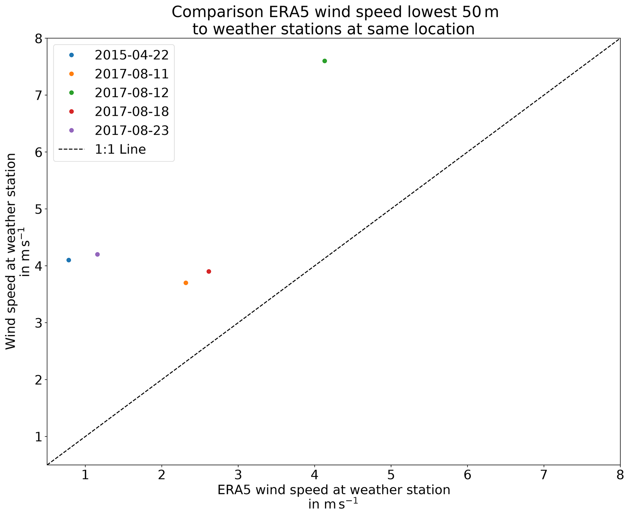
Figure A1Comparison between wind speed averaged over the lowest 50 m above ground for ERA5 data and collocated wind station data. ERA5 data significantly underestimated the wind speed present at a given time.
In a push-broom imager such as AVIRIS-NG, each detector column acts as one separate line detector looking at a different ground scene. Even with very good calibration and characterization (described in Chapman et al., 2019, for AVIRIS-NG), there will still be small differences in the spectra recorded by two different lines. In the retrieval results, this leads to a line-dependent (or column-dependent) difference in the retrieval results called “striping” (see, for example, Fig. 5). To correct this effect, we normalize the , , and for each pixel by the median PSF of its corresponding detector column. We select the median for resilience against outliers which could otherwise have a large impact on the correction
In this section, additional plumes are shown which have been detected in the data but were either too inconsistent or the conditions did not allow for the application of the cross-sectional flux method.
Very interesting observations are the plumes and CH4 accumulations due to open-cast coal mining, as can be seen in Fig. C1. During coal mining, the enclosed methane is released into the environment. For underground mining, the methane concentration in the air in the mining shafts is kept well below the explosion limit by ventilating the shafts with fresh air (Özgen Karacan, 2008). The ventilation shafts then emit the total emissions from the whole mine. In an open coal mine, the emissions may come out diffuse; however, according to Fig. C1, it seems that significant amounts of methane may be emitted from the brim, perhaps during the cutting of the coal.
Additional plumes are shown in Figs. C2 and C3. Those plumes originate from oil and gas infrastructure such as a well pad in the forest and vents. Especially the vents in Fig. C3 are only very faintly visible.
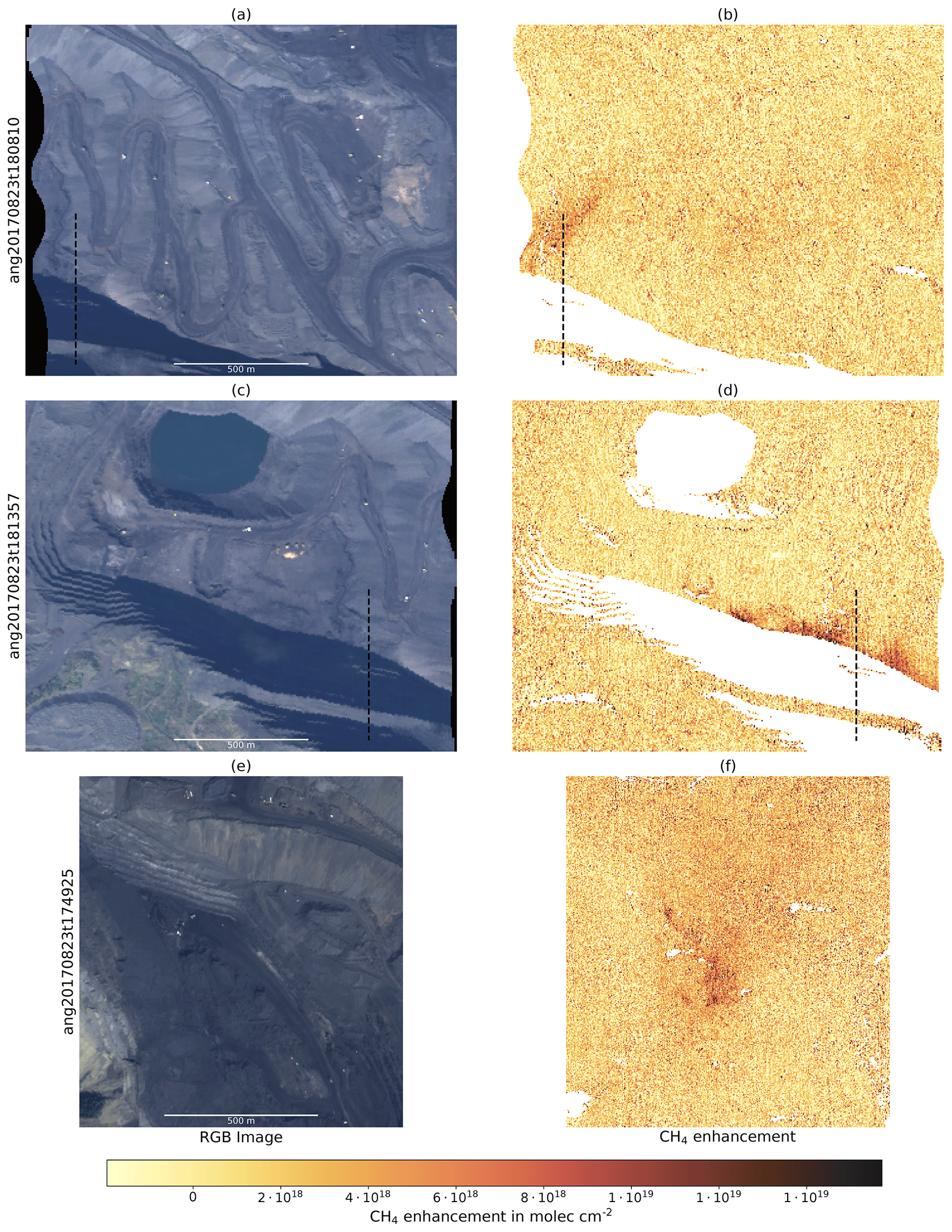
Figure C1Same as Fig. 9 but for methane enhancements after application of the proxy resulting from bituminous coal extraction. The upper two measurements were taken within ∼10 min and show the same brim. The dashed line is plotted on the same location in both images. While in panel (b) a plume emanating from the brim is visible, in panel (d) strong accumulations near the brim are visible. In panel (f), the plume is more diffuse, and the highest enhancements are visible near a brim. However, it is not as clear as in panels (b) and (d) if it really originates from the brim or might be an artifact.
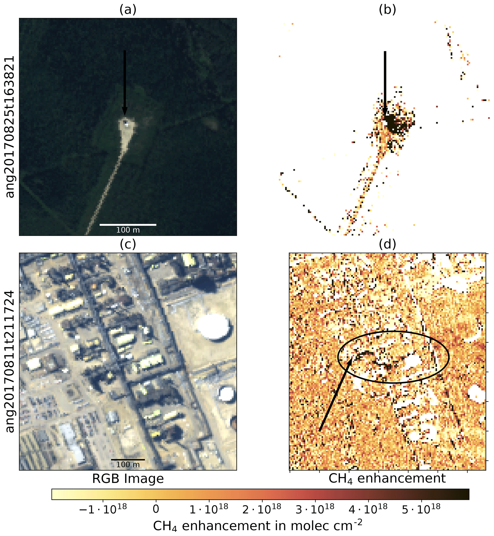
Figure C2Similar to Fig. C1 but for methane enhancements from oil/gas infrastructure. In panels (a) and (b), the emissions originate from a well pad in a forest. Due to the low radiance over the trees, only the well pad itself passes the quality filters. The enhancements seem accumulated, and no clear wind direction is visible. In panels (c) and (d), a facility located at a bitumen extraction site is shown, and the methane plume meanders around the facility.
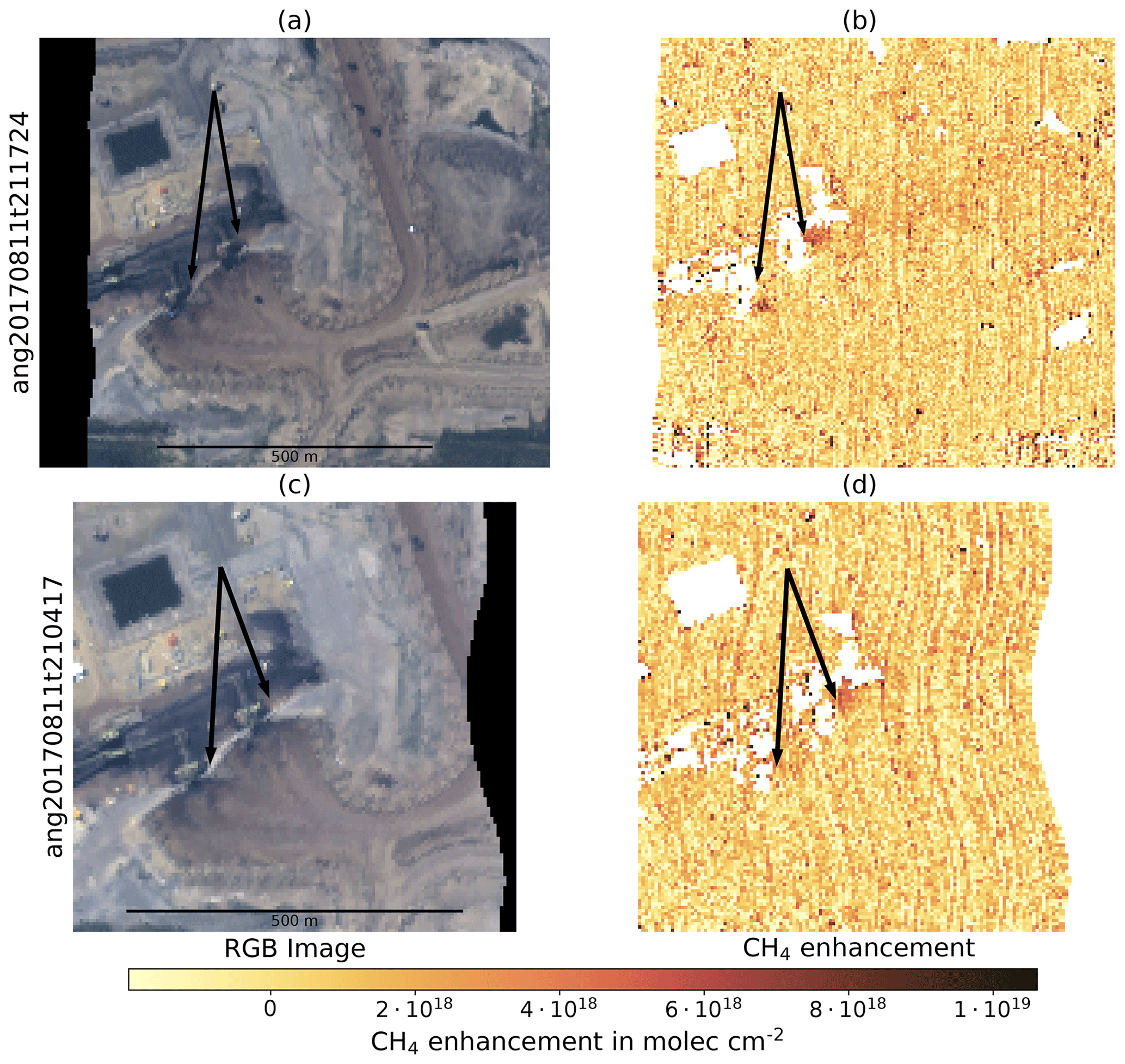
Figure C3Similar to Fig. C1 but for two overpasses over cold vents at a bitumen extraction site. The plumes are only faint, especially for the second overpass (d). In the results, a small striping effect is still visible. The destriping reduces the effect but is not able to totally eliminate it.
In addition to the comparison of IMAP-DOAS and MF for the same plume, we compared MF and WFM-DOAS retrieval results for subregions zoomed in on plumes P1–P4 (see Fig. D1). For the scene P3, the retrievals seem to agree quite well. Especially the higher enhancements correlated with the plume lay near the 1 : 1 line. However, for plumes P1, P2, and P4, there is a bigger discrepancy between MF and WFM-DOAS which can not be explained by the larger scatter alone. The cause for this is currently under investigation.

The AVIRIS-NG data set of the ABoVE campaign is available at https://doi.org/10.3334/ORNLDAAC/1569 (Miller et al., 2019a).
JB contributed to the study design, adapted the retrieval, analyzed the data, and wrote the paper, KG and HB initialized the study, KG and SK contributed to the retrieval adaption, study design, and paper draft, AKT, DRT, and CF helped in data set selection and with the handling of the data, RMD and CEM designed the flight plans and organized and led the flights, and HB and JPB supervised the study, contributing to the scientific objectives and interpretation of results. All authors contributed to the final paper.
The authors declare that they have no conflict of interest.
We would also like to acknowledge the contributions of the AVIRIS flight and instrument teams. The AVIRIS-NG data were collected as part of the Arctic-Boreal Vulnerability Experiment (ABoVE), a NASA Terrestrial Ecology program, and other methane studies were supported by NASA's Earth Science Division. A portion of this work was performed at the Jet Propulsion Laboratory, California Institute of Technology, under contract with NASA. The hourly resolved wind data for P3 and P4 were provided by Alberta Agriculture and Forestry, Alberta Climate Information Service (ACIS), https://acis.alberta.ca (last access: 21 December 2020) for stations Patricia AGCM and Sundre A.
This research has been supported by the BMBF project AIRSPACE MAMAP 2D (grant no. FKZ01LK1701B).
The article processing charges for this open-access publication were covered by the University of Bremen.
This paper was edited by Ilse Aben and reviewed by Luis Guanter and one anonymous referee.
Ayasse, A. K., Thorpe, A. K., Roberts, D. A., Funk, C. C., Dennison, P. E., Frankenberg, C., Steffke, A., and Aubrey, A. D.: Evaluating the effects of surface properties on methane retrievals using a synthetic airborne visible/infrared imaging spectrometer next generation (AVIRIS-NG) image, Remote Sens. Environ., 215, 386–397, https://doi.org/10.1016/j.rse.2018.06.018, 2018. a, b
Baldridge, A., Hook, S., Grove, C., and Rivera, G.: The ASTER spectral library version 2.0, Remote Sens. Environ., 113, 711–715, https://doi.org/10.1016/j.rse.2008.11.007, 2009. a
Berchet, A., Zink, K., Muller, C., Oettl, D., Brunner, J., Emmenegger, L., and Brunner, D.: A cost-effective method for simulating city-wide air flow and pollutant dispersion at building resolving scale, Atmos. Environ., 158, 181–196, https://doi.org/10.1016/j.atmosenv.2017.03.030, 2017. a
Bovensmann, H., Burrows, J. P., Buchwitz, M., Frerick, J., Noël, S., Rozanov, V. V., Chance, K. V., and Goede, A. P. H.: SCIAMACHY: Mission Objectives and Measurement Modes, J. Atmos. Sci., 56, 127–150, https://doi.org/10.1175/1520-0469(1999)056<0127:smoamm>2.0.co;2, 1999. a
Buchwitz, M., Rozanov, V. V., and Burrows, J. P.: A near-infrared optimized DOAS method for the fast global retrieval of atmospheric CH4, CO, CO2, H2O, and N2O total column amounts from SCIAMACHY Envisat-1 nadir radiances, J. Geophys. Res.-Atmos., 105, 15231–15245, https://doi.org/10.1029/2000jd900191, 2000. a
Buchwitz, M., Schneising, O., Reuter, M., Heymann, J., Krautwurst, S., Bovensmann, H., Burrows, J. P., Boesch, H., Parker, R. J., Somkuti, P., Detmers, R. G., Hasekamp, O. P., Aben, I., Butz, A., Frankenberg, C., and Turner, A. J.: Satellite-derived methane hotspot emission estimates using a fast data-driven method, Atmos. Chem. Phys., 17, 5751–5774, https://doi.org/10.5194/acp-17-5751-2017, 2017. a
Burrows, J., Hölzle, E., Goede, A., Visser, H., and Fricke, W.: SCIAMACHY – scanning imaging absorption spectrometer for atmospheric chartography, Acta Astronaut., 35, 445–451, https://doi.org/10.1016/0094-5765(94)00278-T, 1995. a
Chapman, J. W., Thompson, D. R., Helmlinger, M. C., Bue, B. D., Green, R. O., Eastwood, M. L., Geier, S., Olson-Duvall, W., and Lundeen, S. R.: Spectral and Radiometric Calibration of the Next Generation Airborne Visible Infrared Spectrometer (AVIRIS-NG), Remote Sens.-Basel, 11, 2129, https://doi.org/10.3390/rs11182129, 2019. a, b, c, d
Chen, Y., Sun-Mack, S., Arduini, R. F., Trepte, Q., and Minnis, P.: Clear-Sky and Surface Narrowband Albedo Datasets Derived from MODIS Data, https://doi.org/10.1117/12.511180, 2006. a
Copernicus Climate Change Service (C3S): ERA5: Fifth generation of ECMWF atmospheric reanalyses of the global climate, Copernicus Climate Change Service Climate Data Store (CDS), available at: https://cds.climate.copernicus.eu/cdsapp#!/home (last access: 2 December 2020), 2017. a
Cusworth, D. H., Jacob, D. J., Varon, D. J., Chan Miller, C., Liu, X., Chance, K., Thorpe, A. K., Duren, R. M., Miller, C. E., Thompson, D. R., Frankenberg, C., Guanter, L., and Randles, C. A.: Potential of next-generation imaging spectrometers to detect and quantify methane point sources from space, Atmos. Meas. Tech., 12, 5655–5668, https://doi.org/10.5194/amt-12-5655-2019, 2019. a
Cusworth, D. H., Duren, R. M., Thorpe, A. K., Tseng, E., Thompson, D., Guha, A., Newman, S., Foster, K. T., and Miller, C. E.: Using remote sensing to detect, validate, and quantify methane emissions from California solid waste operations, Environ. Res. Lett., 15, 054012, https://doi.org/10.1088/1748-9326/ab7b99, 2020. a
Dlugokencky, E. J.: Globaly Averaged marine surface annual mean growth rate, available at: https://www.esrl.noaa.gov/gmd/ccgg/trends_ch4/ (last access: 5 August 2019), 2018. a, b
Dlugokencky, E. J., Nisbet, E. G., Fisher, R., and Lowry, D.: Global atmospheric methane: budget, changes and dangers, Philos. T. R. Soc. A, 369, 2058–2072, https://doi.org/10.1098/rsta.2010.0341, 2011. a
Duren, R. M., Thorpe, A. K., Foster, K. T., Rafiq, T., Hopkins, F. M., Yadav, V., Bue, B. D., Thompson, D. R., Conley, S., Colombi, N. K., Frankenberg, C., McCubbin, I. B., Eastwood, M. L., Falk, M., Herner, J. D., Croes, B. E., Green, R. O., and Miller, C. E.: California's methane super-emitters, Nature, 575, 180–184, https://doi.org/10.1038/s41586-019-1720-3, 2019. a
Foote, M. D., Dennison, P. E., Thorpe, A. K., Thompson, D. R., Jongaramrungruang, S., Frankenberg, C., and Joshi, S. C.: Fast and Accurate Retrieval of Methane Concentration From Imaging Spectrometer Data Using Sparsity Prior, IEEE T. Geosci. Remote, 58, 6480–6492, https://doi.org/10.1109/tgrs.2020.2976888, 2020. a
Frankenberg, C., Platt, U., and Wagner, T.: Iterative maximum a posteriori (IMAP)-DOAS for retrieval of strongly absorbing trace gases: Model studies for CH4 and CO2 retrieval from near infrared spectra of SCIAMACHY onboard ENVISAT, Atmos. Chem. Phys., 5, 9–22, https://doi.org/10.5194/acp-5-9-2005, 2005. a, b, c
Frankenberg, C., Meirink, J. F., Bergamaschi, P., Goede, A. P. H., Heimann, M., Körner, S., Platt, U., van Weele, M., and Wagner, T.: Satellite chartography of atmospheric methane from SCIAMACHY on board ENVISAT: Analysis of the years 2003 and 2004, J. Geophys. Res., 111, D07303, https://doi.org/10.1029/2005jd006235, 2006. a
Frankenberg, C., Thorpe, A. K., Thompson, D. R., Hulley, G., Kort, E. A., Vance, N., Borchardt, J., Krings, T., Gerilowski, K., Sweeney, C., Conley, S., Bue, B. D., Aubrey, A. D., Hook, S., and Green, R. O.: Airborne methane remote measurements reveal heavy-tail flux distribution in Four Corners region, P. Natl. Acad. Sci. USA, 113, 9734–9739, https://doi.org/10.1073/pnas.1605617113, 2016. a, b, c, d
Gerilowski, K., Tretner, A., Krings, T., Buchwitz, M., Bertagnolio, P. P., Belemezov, F., Erzinger, J., Burrows, J. P., and Bovensmann, H.: MAMAP – a new spectrometer system for column-averaged methane and carbon dioxide observations from aircraft: instrument description and performance analysis, Atmos. Meas. Tech., 4, 215–243, https://doi.org/10.5194/amt-4-215-2011, 2011. a, b
Gordon, I., Rothman, L., Hill, C., Kochanov, R., Tan, Y., Bernath, P., Birk, M., Boudon, V., Campargue, A., Chance, K., Drouin, B., Flaud, J.-M., Gamache, R., Hodges, J., Jacquemart, D., Perevalov, V., Perrin, A., Shine, K., Smith, M.-A., Tennyson, J., Toon, G., Tran, H., Tyuterev, V., Barbe, A., Császár, A., Devi, V., Furtenbacher, T., Harrison, J., Hartmann, J.-M., Jolly, A., Johnson, T., Karman, T., Kleiner, I., Kyuberis, A., Loos, J., Lyulin, O., Massie, S., Mikhailenko, S., Moazzen-Ahmadi, N., Müller, H., Naumenko, O., Nikitin, A., Polyansky, O., Rey, M., Rotger, M., Sharpe, S., Sung, K., Starikova, E., Tashkun, S., Auwera, J. V., Wagner, G., Wilzewski, J., Wcisło, P., Yu, S., and Zak, E.: The HITRAN 2016 molecular spectroscopic database, J. Quant. Spectrosc. Ra., 203, 3–69, https://doi.org/10.1016/j.jqsrt.2017.06.038, 2017. a
Hamlin, L., Green, R. O., Mouroulis, P., Eastwood, M., Wilson, D., Dudik, M., and Paine, C.: Imaging spectrometer science measurements for Terrestrial Ecology: AVIRIS and new developments, 2011 Aerospace Conference, 5–12 March 2011, Big Sky, Montana, USA, 1–7, https://doi.org/10.1109/aero.2011.5747395, 2011. a
Hess, M., Koepke, P., and Schult, I.: Optical Properties of Aerosols and Clouds: The Software Package OPAC, B. Am. Meteorol. Soc. 79, 831–844, https://doi.org/10.1175/1520-0477(1998)079<0831:opoaac>2.0.co;2, 1998. a
Horel, J., Splitt, M., Dunn, L., Pechmann, J., White, B., Ciliberti, C., Lazarus, S., Slemmer, J., Zaff, D., and Burks, J.: MESOWEST: Cooperative Mesonets in the Western United States, B. Am. Meteorol. Soc. 83, 211–226, https://doi.org/10.1175/1520-0477(2002)083<0211:MCMITW>2.3.CO;2, 2002. a
Hu, H., Hasekamp, O., Butz, A., Galli, A., Landgraf, J., Aan de Brugh, J., Borsdorff, T., Scheepmaker, R., and Aben, I.: The operational methane retrieval algorithm for TROPOMI, Atmos. Meas. Tech., 9, 5423–5440, https://doi.org/10.5194/amt-9-5423-2016, 2016. a
Hu, H., Landgraf, J., Detmers, R., Borsdorff, T., de Brugh, J. A., Aben, I., Butz, A., and Hasekamp, O.: Toward Global Mapping of Methane With TROPOMI: First Results and Intersatellite Comparison to GOSAT, Geophys. Res. Lett., 45, 3682–3689, https://doi.org/10.1002/2018gl077259, 2018. a
Hulley, G. C., Duren, R. M., Hopkins, F. M., Hook, S. J., Vance, N., Guillevic, P., Johnson, W. R., Eng, B. T., Mihaly, J. M., Jovanovic, V. M., Chazanoff, S. L., Staniszewski, Z. K., Kuai, L., Worden, J., Frankenberg, C., Rivera, G., Aubrey, A. D., Miller, C. E., Malakar, N. K., Sánchez Tomás, J. M., and Holmes, K. T.: High spatial resolution imaging of methane and other trace gases with the airborne Hyperspectral Thermal Emission Spectrometer (HyTES), Atmos. Meas. Tech., 9, 2393–2408, https://doi.org/10.5194/amt-9-2393-2016, 2016. a
IPCC 2013: climate change 2013: the physical science basis, Contribution of working group I [Stocker, T. F., Qin, D., Plattner, G. K., Tignor, M., Allen, S. K., Boschung, J., Nauels, A., Xia, Y., Bex, B., and Midgley, B. M.] to the fifth assessment report of the intergovernmental panel on climate change, Cambridge University Press, https://doi.org/10.1017/CBO9781107415324, 2013. a
Jongaramrungruang, S., Frankenberg, C., Matheou, G., Thorpe, A. K., Thompson, D. R., Kuai, L., and Duren, R. M.: Towards accurate methane point-source quantification from high-resolution 2D plume imagery, Atmos. Meas. Tech., 12, 6667–6681, https://doi.org/10.5194/amt-12-6667-2019, 2019. a, b
Kerkweg, A. and Jöckel, P.: The 1-way on-line coupled atmospheric chemistry model system MECO(n) – Part 1: Description of the limited-area atmospheric chemistry model COSMO/MESSy, Geosci. Model Dev., 5, 87–110, https://doi.org/10.5194/gmd-5-87-2012, 2012. a
Kokaly, R. F., Clark, R. N., Swayze, G. A., Livo, K. E., Hoefen, T. M., Pearson, N. C., Wise, R. A., Benzel, W. M., Lowers, H. A., Driscoll, R. L., and Klein, A. J.: USGS Spectral Library Version 7, US Geological Survey Data Series 1035, p. 61, https://doi.org/10.3133/ds1035, 2017. a
Krautwurst, S., Gerilowski, K., Jonsson, H. H., Thompson, D. R., Kolyer, R. W., Iraci, L. T., Thorpe, A. K., Horstjann, M., Eastwood, M., Leifer, I., Vigil, S. A., Krings, T., Borchardt, J., Buchwitz, M., Fladeland, M. M., Burrows, J. P., and Bovensmann, H.: Methane emissions from a Californian landfill, determined from airborne remote sensing and in situ measurements, Atmos. Meas. Tech., 10, 3429–3452, https://doi.org/10.5194/amt-10-3429-2017, 2017. a, b, c, d
Krings, T., Gerilowski, K., Buchwitz, M., Reuter, M., Tretner, A., Erzinger, J., Heinze, D., Pflüger, U., Burrows, J. P., and Bovensmann, H.: MAMAP – a new spectrometer system for column-averaged methane and carbon dioxide observations from aircraft: retrieval algorithm and first inversions for point source emission rates, Atmos. Meas. Tech., 4, 1735–1758, https://doi.org/10.5194/amt-4-1735-2011, 2011. a, b, c, d, e, f, g, h
Krings, T., Gerilowski, K., Buchwitz, M., Hartmann, J., Sachs, T., Erzinger, J., Burrows, J. P., and Bovensmann, H.: Quantification of methane emission rates from coal mine ventilation shafts using airborne remote sensing data, Atmos. Meas. Tech., 6, 151–166, https://doi.org/10.5194/amt-6-151-2013, 2013. a, b
Krings, T., Neininger, B., Gerilowski, K., Krautwurst, S., Buchwitz, M., Burrows, J. P., Lindemann, C., Ruhtz, T., Schüttemeyer, D., and Bovensmann, H.: Airborne remote sensing and in situ measurements of atmospheric CO2 to quantify point source emissions, Atmos. Meas. Tech., 11, 721–739, https://doi.org/10.5194/amt-11-721-2018, 2018. a, b
Meerdink, S. K., Hook, S. J., Roberts, D. A., and Abbott, E. A.: The ECOSTRESS spectral library version 1.0, Remote Sens. Environ., 230, 111196, https://doi.org/10.1016/j.rse.2019.05.015, 2019. a
Miller, C. E., Green, R., Thompson, D., Thorpe, A., Eastwood, M., McCubbin, I., Olson-Duvall, W., Bernas, M., Sarture, C., Nolte, S., Rios, L., Hernandez, M., Bue, B., and Lundeenh, S.: ABoVE: Hyperspectral Imagery from AVIRIS-NG, Alaskan and Canadian Arctic, 2017–2018, ORNL DAAC, Oak Ridge, Tennessee, USA, https://doi.org/10.3334/ORNLDAAC/1569, 2019a. a, b, c
Miller, C. E., Griffith, P., Goetz, S., Hoy, E., Pinto, N., McCubbin, I., Thorpe, A. K., Hofton, M. M., Hodkinson, D. J., Hansen, C., Woods, J., Larsen, E. K., Kasischke, E. S., and Margolis, H. A.: An overview of ABoVE airborne campaign data acquisitions and science opportunities, Environ. Res. Lett., 14, 080201, https://doi.org/10.1088/1748-9326/ab0d44, 2019b. a, b
Minola, L., Zhang, F., Azorin-Molina, C., Pirooz, A. A. S., Flay, R. G. J., Hersbach, H., and Chen, D.: Near-surface mean and gust wind speeds in ERA5 across Sweden: towards an improved gust parametrization, Clim. Dynam., 55, 887–907, https://doi.org/10.1007/s00382-020-05302-6, 2020. a
Nisbet, E. G., Manning, M. R., Dlugokencky, E. J., Fisher, R. E., Lowry, D., Michel, S. E., Myhre, C. L., Platt, S. M., Allen, G., Bousquet, P., Brownlow, R., Cain, M., France, J. L., Hermansen, O., Hossaini, R., Jones, A. E., Levin, I., Manning, A. C., Myhre, G., Pyle, J. A., Vaughn, B. H., Warwick, N. J., and White, J. W. C.: Very Strong Atmospheric Methane Growth in the 4 Years 2014–2017: Implications for the Paris Agreement, Global Biochem. Cy., 33, 318–342, https://doi.org/10.1029/2018gb006009, 2019. a
NOAA (National Oceanic and Atmospheric Administration): US standard atmosphere, vol. 76, National Oceanic and Atmospheric Administration, Washington, D.C., USA, 227 pp., 1976. a
Özgen Karacan, C.: Modeling and prediction of ventilation methane emissions of US longwall mines using supervised artificial neural networks, Int. J. Coal Geol., 73, 371–387, https://doi.org/10.1016/j.coal.2007.09.003, 2008. a
Pandey, S., Gautam, R., Houweling, S., van der Gon, H. D., Sadavarte, P., Borsdorff, T., Hasekamp, O., Landgraf, J., Tol, P., van Kempen, T., Hoogeveen, R., van Hees, R., Hamburg, S. P., Maasakkers, J. D., and Aben, I.: Satellite observations reveal extreme methane leakage from a natural gas well blowout, P. Natl. Acad. Sci. USA, 201908712, https://doi.org/10.1073/pnas.1908712116, 2019. a
Paris Agreement: United Nations Framework Convention on Climate Change, Paris, France, 2015. a
Reuter, M., Buchwitz, M., Schneising, O., Hase, F., Heymann, J., Guerlet, S., Cogan, A. J., Bovensmann, H., and Burrows, J. P.: A simple empirical model estimating atmospheric CO2 background concentrations, Atmos. Meas. Tech., 5, 1349–1357, https://doi.org/10.5194/amt-5-1349-2012, 2012. a
Reuter, M., Buchwitz, M., Schneising, O., Noël, S., Bovensmann, H., Burrows, J. P., Boesch, H., Di Noia, A., Anand, J., Parker, R. J., Somkuti, P., Wu, L., Hasekamp, O. P., Aben, I., Kuze, A., Suto, H., Shiomi, K., Yoshida, Y., Morino, I., Crisp, D., O'Dell, C. W., Notholt, J., Petri, C., Warneke, T., Velazco, V. A., Deutscher, N. M., Griffith, D. W. T., Kivi, R., Pollard, D. F., Hase, F., Sussmann, R., Té, Y. V., Strong, K., Roche, S., Sha, M. K., De Mazière, M., Feist, D. G., Iraci, L. T., Roehl, C. M., Retscher, C., and Schepers, D.: Ensemble-based satellite-derived carbon dioxide and methane column-averaged dry-air mole fraction data sets (2003–2018) for carbon and climate applications, Atmos. Meas. Tech., 13, 789–819, https://doi.org/10.5194/amt-13-789-2020, 2020. a
Rozanov, V., Dinter, T., Rozanov, A., Wolanin, A., Bracher, A., and Burrows, J.: Radiative transfer modeling through terrestrial atmosphere and ocean accounting for inelastic processes: Software package SCIATRAN, J. Quant. Spectrosc. Ra., 194, 65–85, https://doi.org/10.1016/j.jqsrt.2017.03.009, 2017. a
Saunois, M., Bousquet, P., Poulter, B., Peregon, A., Ciais, P., Canadell, J. G., Dlugokencky, E. J., Etiope, G., Bastviken, D., Houweling, S., Janssens-Maenhout, G., Tubiello, F. N., Castaldi, S., Jackson, R. B., Alexe, M., Arora, V. K., Beerling, D. J., Bergamaschi, P., Blake, D. R., Brailsford, G., Brovkin, V., Bruhwiler, L., Crevoisier, C., Crill, P., Covey, K., Curry, C., Frankenberg, C., Gedney, N., Höglund-Isaksson, L., Ishizawa, M., Ito, A., Joos, F., Kim, H.-S., Kleinen, T., Krummel, P., Lamarque, J.-F., Langenfelds, R., Locatelli, R., Machida, T., Maksyutov, S., McDonald, K. C., Marshall, J., Melton, J. R., Morino, I., Naik, V., O'Doherty, S., Parmentier, F.-J. W., Patra, P. K., Peng, C., Peng, S., Peters, G. P., Pison, I., Prigent, C., Prinn, R., Ramonet, M., Riley, W. J., Saito, M., Santini, M., Schroeder, R., Simpson, I. J., Spahni, R., Steele, P., Takizawa, A., Thornton, B. F., Tian, H., Tohjima, Y., Viovy, N., Voulgarakis, A., van Weele, M., van der Werf, G. R., Weiss, R., Wiedinmyer, C., Wilton, D. J., Wiltshire, A., Worthy, D., Wunch, D., Xu, X., Yoshida, Y., Zhang, B., Zhang, Z., and Zhu, Q.: The global methane budget 2000–2012, Earth Syst. Sci. Data, 8, 697–751, https://doi.org/10.5194/essd-8-697-2016, 2016. a
Saunois, M., Stavert, A. R., Poulter, B., Bousquet, P., Canadell, J. G., Jackson, R. B., Raymond, P. A., Dlugokencky, E. J., Houweling, S., Patra, P. K., Ciais, P., Arora, V. K., Bastviken, D., Bergamaschi, P., Blake, D. R., Brailsford, G., Bruhwiler, L., Carlson, K. M., Carrol, M., Castaldi, S., Chandra, N., Crevoisier, C., Crill, P. M., Covey, K., Curry, C. L., Etiope, G., Frankenberg, C., Gedney, N., Hegglin, M. I., Höglund-Isaksson, L., Hugelius, G., Ishizawa, M., Ito, A., Janssens-Maenhout, G., Jensen, K. M., Joos, F., Kleinen, T., Krummel, P. B., Langenfelds, R. L., Laruelle, G. G., Liu, L., Machida, T., Maksyutov, S., McDonald, K. C., McNorton, J., Miller, P. A., Melton, J. R., Morino, I., Müller, J., Murguia-Flores, F., Naik, V., Niwa, Y., Noce, S., O'Doherty, S., Parker, R. J., Peng, C., Peng, S., Peters, G. P., Prigent, C., Prinn, R., Ramonet, M., Regnier, P., Riley, W. J., Rosentreter, J. A., Segers, A., Simpson, I. J., Shi, H., Smith, S. J., Steele, L. P., Thornton, B. F., Tian, H., Tohjima, Y., Tubiello, F. N., Tsuruta, A., Viovy, N., Voulgarakis, A., Weber, T. S., van Weele, M., van der Werf, G. R., Weiss, R. F., Worthy, D., Wunch, D., Yin, Y., Yoshida, Y., Zhang, W., Zhang, Z., Zhao, Y., Zheng, B., Zhu, Q., Zhu, Q., and Zhuang, Q.: The Global Methane Budget 2000–2017, Earth Syst. Sci. Data, 12, 1561–1623, https://doi.org/10.5194/essd-12-1561-2020, 2020. a
Scafutto, R. D. M., de Souza Filho, C. R., Riley, D. N., and de Oliveira, W. J.: Evaluation of thermal infrared hyperspectral imagery for the detection of onshore methane plumes: Significance for hydrocarbon exploration and monitoring, Int. J. Appl. Earth Obs., 64, 311–325, https://doi.org/10.1016/j.jag.2017.07.002, 2018. a
Schaefer, H.: On the Causes and Consequences of Recent Trends in Atmospheric Methane, Curr. Clim. Change Rep., 5, 259–274, https://doi.org/10.1007/s40641-019-00140-z, 2019. a
Schneising, O., Buchwitz, M., Burrows, J. P., Bovensmann, H., Reuter, M., Notholt, J., Macatangay, R., and Warneke, T.: Three years of greenhouse gas column-averaged dry air mole fractions retrieved from satellite – Part 1: Carbon dioxide, Atmos. Chem. Phys., 8, 3827–3853, https://doi.org/10.5194/acp-8-3827-2008, 2008. a
Schneising, O., Buchwitz, M., Burrows, J. P., Bovensmann, H., Bergamaschi, P., and Peters, W.: Three years of greenhouse gas column-averaged dry air mole fractions retrieved from satellite – Part 2: Methane, Atmos. Chem. Phys., 9, 443–465, https://doi.org/10.5194/acp-9-443-2009, 2009. a, b
Schneising, O., Buchwitz, M., Reuter, M., Bovensmann, H., Burrows, J. P., Borsdorff, T., Deutscher, N. M., Feist, D. G., Griffith, D. W. T., Hase, F., Hermans, C., Iraci, L. T., Kivi, R., Landgraf, J., Morino, I., Notholt, J., Petri, C., Pollard, D. F., Roche, S., Shiomi, K., Strong, K., Sussmann, R., Velazco, V. A., Warneke, T., and Wunch, D.: A scientific algorithm to simultaneously retrieve carbon monoxide and methane from TROPOMI onboard Sentinel-5 Precursor, Atmos. Meas. Tech., 12, 6771–6802, https://doi.org/10.5194/amt-12-6771-2019, 2019. a, b, c
Thompson, D. R., Leifer, I., Bovensmann, H., Eastwood, M., Fladeland, M., Frankenberg, C., Gerilowski, K., Green, R. O., Kratwurst, S., Krings, T., Luna, B., and Thorpe, A. K.: Real-time remote detection and measurement for airborne imaging spectroscopy: a case study with methane, Atmos. Meas. Tech., 8, 4383–4397, https://doi.org/10.5194/amt-8-4383-2015, 2015. a, b, c, d
Thompson, D. R., Thorpe, A. K., Frankenberg, C., Green, R. O., Duren, R., Guanter, L., Hollstein, A., Middleton, E., Ong, L., and Ungar, S.: Space-based remote imaging spectroscopy of the Aliso Canyon CH4 superemitter, Geophys. Res. Lett., 43, 6571–6578, https://doi.org/10.1002/2016gl069079, 2016. a
Thorpe, A. K., Roberts, D. A., Bradley, E. S., Funk, C. C., Dennison, P. E., and Leifer, I.: High resolution mapping of methane emissions from marine and terrestrial sources using a Cluster-Tuned Matched Filter technique and imaging spectrometry, Remote Sens. Environ., 134, 305–318, https://doi.org/10.1016/j.rse.2013.03.018, 2013. a
Thorpe, A. K., Frankenberg, C., and Roberts, D. A.: Retrieval techniques for airborne imaging of methane concentrations using high spatial and moderate spectral resolution: application to AVIRIS, Atmos. Meas. Tech., 7, 491–506, https://doi.org/10.5194/amt-7-491-2014, 2014. a
Thorpe, A. K., Frankenberg, C., Aubrey, A., Roberts, D., Nottrott, A., Rahn, T., Sauer, J., Dubey, M., Costigan, K., Arata, C., Steffke, A., Hills, S., Haselwimmer, C., Charlesworth, D., Funk, C., Green, R., Lundeen, S., Boardman, J., Eastwood, M., Sarture, C., Nolte, S., Mccubbin, I., Thompson, D., and McFadden, J.: Mapping methane concentrations from a controlled release experiment using the next generation airborne visible/infrared imaging spectrometer (AVIRIS-NG), Remote Sens. Environ., 179, 104–115, https://doi.org/10.1016/j.rse.2016.03.032, 2016a. a, b
Thorpe, A. K., Frankenberg, C., Green, R. O., Thompson, D. R., Aubrey, A. D., Mouroulis, P., Eastwood, M. L., and Matheou, G.: The Airborne Methane Plume Spectrometer (AMPS): Quantitative imaging of methane plumes in real time, 2016 IEEE Aerospace Conference, 5–12 March 2016, Big Sky, Montana, USA, 1–14, https://doi.org/10.1109/aero.2016.7500756, 2016b. a, b
Thorpe, A. K., Frankenberg, C., Thompson, D. R., Duren, R. M., Aubrey, A. D., Bue, B. D., Green, R. O., Gerilowski, K., Krings, T., Borchardt, J., Kort, E. A., Sweeney, C., Conley, S., Roberts, D. A., and Dennison, P. E.: Airborne DOAS retrievals of methane, carbon dioxide, and water vapor concentrations at high spatial resolution: application to AVIRIS-NG, Atmos. Meas. Tech., 10, 3833–3850, https://doi.org/10.5194/amt-10-3833-2017, 2017. a, b, c, d
Thorpe, A. K., Duren, R. M., Conley, S., Prasad, K. R., Bue, B. D., Yadav, V., Foster, K. T., Rafiq, T., Hopkins, F. M., Smith, M. L., Fischer, M. L., Thompson, D. R., Frankenberg, C., McCubbin, I. B., Eastwood, M. L., Green, R. O., and Miller, C. E.: Methane emissions from underground gas storage in California, Environ. Res. Lett., 15, 045005, https://doi.org/10.1088/1748-9326/ab751d, 2020. a
Varon, D. J., McKeever, J., Jervis, D., Maasakkers, J. D., Pandey, S., Houweling, S., Aben, I., Scarpelli, T., and Jacob, D. J.: Satellite Discovery of Anomalously Large Methane Point Sources From Oil/Gas Production, Geophys. Res. Lett., 46, 13507–13516, https://doi.org/10.1029/2019gl083798, 2019. a, b
Veefkind, J., Aben, I., McMullan, K., Förster, H., de Vries, J., Otter, G., Claas, J., Eskes, H., de Haan, J., Kleipool, Q., van Weele, M., Hasekamp, O., Hoogeveen, R., Landgraf, J., Snel, R., Tol, P., Ingmann, P., Voors, R., Kruizinga, B., Vink, R., Visser, H., and Levelt, P.: TROPOMI on the ESA Sentinel-5 Precursor: A GMES mission for global observations of the atmospheric composition for climate, air quality and ozone layer applications, Remote Sens. Environ., 120, 70–83, https://doi.org/10.1016/j.rse.2011.09.027, 2012. a
White, W., Anderson, J., Blumenthal, D., Husar, R., Gillani, N., Husar, J., and Wilson, W.: Formation and transport of secondary air pollutants: ozone and aerosols in the St. Louis urban plume, Science, 194, 187–189, https://doi.org/10.1126/science.959846, 1976. a
Wildmann, N., Päschke, E., Roiger, A., and Mallaun, C.: Towards improved turbulence estimation with Doppler wind lidar velocity-azimuth display (VAD) scans, Atmos. Meas. Tech., 13, 4141–4158, https://doi.org/10.5194/amt-13-4141-2020, 2020. a
Wood Buffalo Environmental Association: Ambient Air Monitoring Station Site Documentation – AMS 19 Firebag, available at: https://wbea.org/stations/firebag/, last access: 21 December 2020. a
Data provided by Alberta Agriculture and Forestry, Alberta Climate Information Service (ACIS) https://acis.alberta.ca (last access: 21 December 2020).
- Abstract
- Introduction
- Instrument and data sets
- Adaption of WFM-DOAS algorithm to AVIRIS-NG measurements
- Detection and inversion of plumes
- Discussion
- Summary and conclusions
- Appendix A: Comparison of weather station wind data with ERA5 50 m height average data
- Appendix B: Striping effect
- Appendix C: Other detected CH4 plumes
- Appendix D: Additional comparison between MF and WFM-DOAS
- Data availability
- Author contributions
- Competing interests
- Acknowledgements
- Financial support
- Review statement
- References