A novel machine learning retrieval for the detection of ice crystal icing conditions based on geostationary satellite imagery

High ice water content (HIWC) conditions are a concern for aviation as the ingestion of ice particles in the jet engines can induce ice crystal icing (ICI), which results in performance loss and damage. To constantly monitor these conditions, retrievals for the detection of ICI were recently developed based on geostationary satellite imagery, but their calibration is limited to targeted flight campaigns or scattered samplings from ICI events databases. In this work, we close this gap, using exclusively remote sensing data to develop and assess a new retrieval for potential ICI conditions.

Cloud IWC measurements are provided from the synergy of radar and lidar (DARDAR) on board the polar-orbiting satellites CloudSat and CALIPSO. HIWC conditions (IWC≥0.5 g m⁻³) at typical cruise altitudes are used as the proxy for areas with potential ICI formation. The HIWC conditions predictors are taken from a combination of observations and retrievals of the geostationary satellite Meteosat Second Generation (MSG). A random forest is trained and tested based on the collocated dataset of active and passive measurements during the summer months of 2013 and 2015, covering the European domain. The input predictors are the brightness temperature difference between the MSG channels at 6.2 and 10.8 µm wavelengths, the visible channel at 0.6 µm wavelength, the cloud optical thickness at 0.6 µm wavelength, and four convection metrics related to the distance to the closest convective cell, area extent of the convective cells, and convection density in the pixel surroundings. Over Europe, 83 % of HIWC conditions measured in the DARDAR dataset are correctly detected. The associated false alarm rate is 51 %. The retrieval is further tested with the ICI events database reported by Lufthansa. Four out of seven events are correctly detected. In conclusion, the retrieval achieves performances comparable to previously developed retrievals. An operational application would enable aircraft rerouting around areas with high ICI probability.

1 Introduction

Ice Crystal Icing (ICI) is a phenomenon that aircraft may encounter when flying through cloudy regions with high ice crystal concentrations. These regions are mostly found close to deep convection, in particular within tropical mesoscale convective systems (MCSs). In such systems, pilots can easily avoid strong updrafts, as onboard radars can detect embedded precipitation based on its high reflectivity signal, or available satellite-based nowcasting of severe convection (NCS-A, Müller et al., 2022) can issue early warnings. However, regions outside the main updraft may not be affected by nowcasting warnings and they can still contain high ice concentrations despite having little to no radar reflectivity due to the presence of non-precipitating ice particles (Gayet et al., 2012); this is where ICI events can occur because ice particles can build up inside the engine and lead to performance loss and damage (Grzych, 2010; Grzych et al., 2015; Bravin et al., 2015; Haggerty et al., 2019), or they can clog the pitot tube which in turns result into a wrongful transmission of information to the autoflight system; this latter occurrence has caused two fatal accidents in recent years (Ayra et al., 2020). Because those failures can happen in high ice concentration regions, on-board sensor anomalies, as for example the total air temperature (TAT) anomalies, are often used as precursors for engine failures (Haggerty et al., 2016; Rodríguez-Sanz et al., 2018). In contrast with convection patterns, no clear diurnal trends are found globally; however, a seasonal correlation is observed between local convective active seasons and ICI events (Bravin et al., 2015).

High ice water content (HIWC) conditions are often used as a proxy for potential ICI occurrence. For these conditions, a threshold ranging between 0.5–1.0 g m⁻³ is chosen in earlier studies, although a standard value is still under debate because exposure times and engine types might also affect ICI occurrence (de Laat et al., 2017; Yost et al., 2018; Haggerty et al., 2019, 2020; Bedka et al., 2020).

Aircraft manufacturers and airlines have collected ICI events in databases to analyze the importance of the phenomenon. Bravin et al. (2015) present a Boeing database that included 162 events over 12 years. de Laat et al. (2017) construct a database from Airbus containing 59 events, without specifying their time frame. Here, a collection of 100 events from Lufthansa flights during 2016 is considered (Sect. 2.4) to analyze a subset of ICI events as case studies (Sect. 4.2). The worldwide number of ICI events and their impact on engine performance highlights the relevance of the issue to air traffic safety.

The importance of this problem led to the execution of flight campaigns to measure in situ cloud microphysical properties during such events. A combination of specifically designed probes, sensors, and radar instruments was deployed to measure high ice concentrations, particle size distributions, and cloud vertical profiles, respectively. These campaigns are:

• the HAIC-HIWC flight campaign, Darwin, Australia 2014, where HAIC stands for “high altitude ice crystal”;

• the HAIC-HIWC II flight campaign, Cayenne, French-Guiana 2015;

• the HAIC-RADAR flight campaign, Fort Lauderdale, Florida 2015;

• the HAIC-RADAR II flight campaign, Fort Lauderdale, Florida 2018.

The problem's relevance and the availability of new in situ measurements triggered activities in the research area of HIWC conditions detection products from satellites. Indeed, the following retrievals were developed:

• Grzych et al. (2015) develop a 3D HIWC mask exploiting infrared (IR) channels from geostationary satellite imagery combined with numerical weather prediction (NWP) wind fields at different heights and the tropopause level (ECMWF-ERA5, Hersbach et al., 2020). The algorithm is tested with the HAIC-HIWC flight campaign case studies, which are used as ground truth. While a clear correlation between the mask and the in situ measured HIWC conditions is found, the algorithm tends to overestimate the areas affected by this phenomenon, but no performance metrics are reported;

• de Laat et al. (2017) approach the problem by manually setting thresholds on retrieved cloud microphysical variables from geostationary satellite imagery. These thresholds are calibrated using case studies in the Airbus dataset and verified with the synergistic space-borne lidar-radar dataset (DARDAR), derived from active remote sensing measurements on polar-orbiting satellites that include, among others, IWC. The algorithm achieves a probability of detection (POD) of 0.59 but with an associated false alarm rate (FAR) of 0.52;

• Yost et al. (2018) use a combination of geostationary satellite imagery and retrieved cloud optical properties. The considered input variables are associated with a corresponding value of IWC according to a statistical fit performed by collocating the satellite data with flight campaign measurements. This information is translated into a HIWC probability using fuzzy logic. The algorithm is verified with the HAIC-HIWC, HAIC-HIWC II, and HIWC-RADAR flight campaigns, achieving a POD of 0.75 and a FAR of 0.35 during daytime. Reported nighttime performances are inferior (POD: 0.62, FAR: 0.35) because of the lack of cloud optical properties;

• Haggerty et al. (2020) integrate a multitude of data sources, like satellites, on-ground radar, and NWP data. Particle swarm optimization is used to select a subset of variables of interest, which are then combined via fuzzy logic to produce the HIWC probability. The retrieval is verified with the HAIC-HIWC, HAIC-HIWC II, and HIWC-RADAR II flight campaigns, achieving a POD of 0.86 and a FAR of 0.51.

When training potential ICI detection retrievals, a significant amount of in situ HIWC measurements should be considered for statistical significance. Dedicated research flight campaigns are often geographically limited, and they specifically target HIWC conditions. This may introduce a bias when extrapolating from a local to a global context (Haggerty et al., 2020).

While in situ HIWC measurements are the best data to assess potential ICI conditions in convective clouds, alternative approaches exploiting remote sensing measurements can be implemented if one wants to increase the training samples. For operational monitoring, geostationary satellites are used due to their wide field of view and high temporal resolution. Polar-orbiting satellites' active observations cannot be directly applied in operational scenarios because of their small field of view and low repetition time. This work demonstrates the feasibility of a detection method for potential ICI from geostationary satellite observations based on machine learning techniques and trained with the DARDAR dataset as ground truth.

The paper contains a description of the combination of data used to train the ICI detection retrieval in Sect. 2. Next, we describe how the machine learning techniques are applied for the ICI detection task in Sect. 3. In Sect. 4, we present the results validated with active remote sensing data and Lufthansa's ICI database. Finally, in Sect. 5 we summarize the results on the retrieval's performance and discuss its main limitations.

2 Datasets

The ICI retrieval developed in this study relies on physical quantities measured and retrieved by passive instruments on board geostationary satellites, called “predictors” hereafter. The geostationary satellite and the corresponding retrievals employed are presented in Sect. 2.1. The DARDAR dataset is presented in Sect. 2.2 because this contained our ground truth data for IWC measurements of cloud profiles. Lastly, it is important to establish the spatial and temporal distribution of selected in-service ICI events, analyzed in Sect. 2.4.

2.1 MSG and MSG-based retrievals

The predictors' source for this work is the geostationary satellite Meteosat Second Generation (MSG) because it guarantees a continuous spatial coverage of Europe. MSG is equipped with the Spinning Enhanced Visible and Infrared Imager (SEVIRI) that measures reflectance and radiance in the visible and infrared range, thanks to its 11 narrow-band channels and one high-resolution visible (HRV) broadband channel. SEVIRI provides a 3712 pixels×3712 pixels image of the Earth disk with a 3 km×3 km resolution at the nadir. The temporal resolution is 15 min, with a rapid scan service (RSS) available for a subset of the Northern Hemisphere, where images are produced every 5 min (Schmetz et al., 2002). Besides SEVIRI channels, we also use ice cloud properties retrievals based on SEVIRI. The considered retrievals for this study are developed in-house, because of our expertise in their strengths and limitations and because of their availability to us. Nevertheless, in one example we have applied our algorithm using alternative products as input: optical thickness from EUMETSAT and convective cloud information from TOOCAN. This is demonstrated in Sect. 4.4. The ice cloud properties are used as predictors for our ICI retrieval, so the corresponding geostationary-based retrievals are briefly discussed below.

2.1.1 CiPS

CiPS (Cirrus Properties from SEVIRI), developed and characterized by Strandgren et al. (2017a, b), detects thin cirrus clouds from MSG and determines ice optical thickness, ice water path, and cloud top height. The detection is based on Artificial Neural Networks trained with CALIPSO lidar data as ground truth. The training and validation datasets cover the entire SEVIRI disc and the period between 2007–2013, containing close to 50 million data points. The lidar signal experiences strong attenuation when interacting with clouds; therefore, it is considered saturated and thus unreliable whenever there is no backscattering from the surface. This limited CiPS to thin cirrus cloud detection with an optical thickness of approximately below 3. When validated against CALIPSO, CiPS detects correctly 95 % of all cirrus clouds with optical thickness of 1.0, while for thinner cirrus clouds with optical thickness of 0.1, the proportion of detected cirrus over all cirrus is 71 %. The best optical thickness estimation is obtained in the range between 0.35–1.7 with a deviation of less than 50 % from CALIPSO's measurements. The detection exploits SEVIRI thermal channels, regional maximum and averaged brightness temperatures in the infrared and water vapor channels, and surface skin temperatures from NWP global reanalysis (Hersbach et al., 2020).

2.1.2 APICS

APICS (Algorithm for the Physical Interpretation of Clouds with SEVIRI Bugliaro et al., 2011) discriminates cloud phase and microphysical properties from MSG. In particular, cloud optical thickness and effective radius (ranging from 5 to 25 µm for water clouds and from 6 to 84 µm for ice clouds) are retrieved using a look-up table approach based on radiative transfer calculations, which exploits the visible channel at 0.6 µm wavelength, and the near-infrared channel at 1.6 µm.

CiPS and APICS thus analyze similar cloud optical and microphysical characteristics, but they perform best in different situations. CiPS is better suited for thin cirrus clouds analysis, both during day and nighttime. APICS has a wider scope, covering both ice and water clouds of any thickness, but it is limited to daytime due to its rule-based approach on visible and near-infrared channels. Both retrievals are used in this study, because they may provide candidate precursors of high ice water content conditions. The suitability of these retrievals for this task has been discussed in Sect. 3.2

2.1.3 Cb-TRAM

Cb-TRAM (Zinner et al., 2008, 2013) enables the detection and tracking of convective cells from geostationary satellite imagery. It relies on the HRV, infrared 10.8 µm, and water vapor window 6.2 µm channels. Cloud motion and development can be detected through the disparities between two consecutive satellite images. The algorithm can also discriminate different convection development stages: “Stage 1” denotes convection initiation, “Stage 2” rapid vertical development through cloud tops cooling, and “Stage 3” indicates mature convective cells.

2.2 DARDAR

DARDAR description

The DARDAR-CLOUD products (Delanoë, 2023a) developed by (Delanoë and Hogan, 2008) exploit the synergy of space-borne data from radar and lidar of the A-train satellite constellation to retrieve ice cloud properties. The A-Train constellation is a group of satellites that use the sun-synchronous orbit at 705 km altitude. CloudSat was equipped with a radar operating in the 94 GHz band, whose aim was to characterize cloud vertical profiles of cloud water and ice contents (Stephens et al., 2002). The lidar on board CALIPSO operated at 532 and 1064 nm wavelengths. CALIPSO provided cloud characterization as a function of height and water and ice content (Winker et al., 2003). These satellites were launched on 28 April 2006 (Delanoë and Hogan, 2010).

The DARDAR-CLOUD products exploit the different sensitivities of the instruments in a synergistic approach. The radar is less sensitive to small particles, but it has a higher penetration capability within thick clouds; the lidar is more sensitive to optically thin clouds, but it is affected by rapid attenuation, while the infrared radiometer can only estimate bulk cloud properties (Delanoë and Hogan, 2010). For this reason, IWC, effective radius, and particle size distributions are retrieved with a variational method that efficiently combines radar and lidar measurements (Delanoë and Hogan, 2008). The DARDAR products are collocated to the CloudSat horizontal resolution of 1.4 km (Stephens et al., 2002) and CALIPSO vertical resolution of 60 m (Delanoë and Hogan, 2010).

2.3 DARDAR-MSG collocation and ICI proxy selection

For our ICI retrieval, we consider DARDAR measurements as ground truth. Therefore, in the first step, we need to collocate the SEVIRI and DARDAR measurements. In the following, we refer to “DARDAR profile” or simply “profile” as the vertical cross-section of clouds as retrieved from the DARDAR dataset. This corresponds to the atmospheric column encompassed in the field of view of one radar-lidar pixel. Instead, we refer to the “DARDAR trajectory” as the DARDAR footprint on the surface in terms of longitude/latitude coordinates.

The DARDAR trajectories have a finer along-track resolution than the geostationary grid. MSG and DARDAR data are combined following the approach described by Mayer et al. (2023). Satellite observations are collocated by exploiting longitude, latitude, cloud top height, and observation times. Cloud top height allows us to correct the parallax effect arising from the different observation geometry of geostationary and polar-orbiting satellites. DARDAR profiles are coarsened to the MSG grid by averaging all profiles within an MSG pixel at each DARDAR height level.

Then, in each averaged profile, we check for HIWC, i.e. IWC≥0.5 g m⁻³, in an altitude range that is relevant for air traffic. We consider only cruise levels between 9000 m and 13 000 m (defined in Sect. 2.4). Figure 1 illustrates the mapping process. Panel (a) showcases the DARDAR IWC profiles coarsened to the MSG grid along the satellite track. HIWC areas are represented with the blue shading. If the maximum IWC value within the cruise levels in the DARDAR IWC profile exceeds the HIWC threshold, the HIWC flag is assigned to the corresponding pixel. Panel (b) depicts the brightness temperature from SEVIRI at 10.8 µm with the corresponding DARDAR trajectory with its longitude/latitude coordinates, the maximum IWC values for each pixel, and the HIWC flag, if applicable. The HIWC flag was used as the target variable to train the machine learning algorithm (Sect. 3).

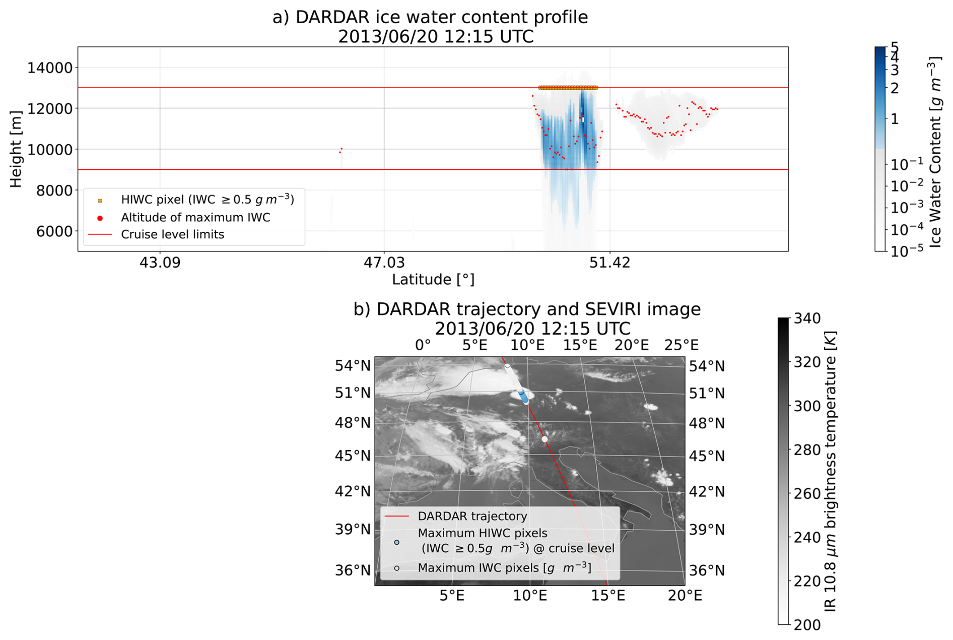
Figure 1 (a) mapping from the DARDAR vertically-resolved IWC information to the HIWC flag associated with the geostationary grid pixel. (b) SEVIRI brightness temperature at 10.8 µm wavelength with the DARDAR trajectory associated with (a).

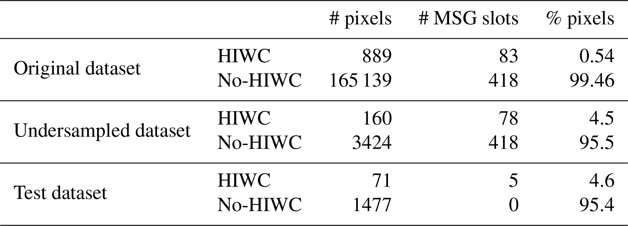
We consider June, July, August, and September 2013 and June, July, and August 2015. Summer months were selected because of the seasonal convective activity peak in Europe. Years 2013 and 2015 are selected because they lie within the time window where DARDAR and a single MSG platform (MSG-3) overlap (from 2013 to 2017) to avoid differences that may arise due to different instrument calibrations (Strandgren et al., 2017a; Mayer et al., 2023; Piontek et al., 2023). The collocated dataset results in 165 139 collocations, 889 of them flagged as HIWC pixels (see Table 1).

Table 1 Proportion of HIWC events vs. no-HIWC events for the original and undersampled dataset. The MSG slot is a single MSG scene containing one DARDAR trajectory. The MSG slot is flagged with HIWC if the corresponding DARDAR trajectory contains at least one HIWC sample; otherwise, it is flagged as no-HIWC. The undersampled dataset excludes five DARDAR trajectories with at least one HIWC pixel that are left out to test the model.

Convection-related metrics from Cb-TRAM

DARDAR trajectories seldom overlap with convective cells as detected by Cb-TRAM. Therefore, additional convection-related metrics are used. The time spent by an aircraft within a HIWC region seems to play a role in the onset of ICI events (Bravin et al., 2015), thus, information about the areal extent of convective cells may be useful during the learning process. To this end, convection-related variables (shown in Fig. 2) are derived from the Cb-TRAM scene:

• distance from the trajectory point to the closest convective cell;

• area size of the closest convective cell, in terms of pixels and km². Since organized convective systems, such as MCSs, are defined as cumulonimbus clouds able to generate contiguous precipitation areas in the order of 100 km (Markowski and Richardson, 2010), this information is useful to assess whether detected cells belong to such organized systems, or if they are associated with single and multi-cell convection, that are generally characterized by a smaller area extent;

• number of convective cells within a 100 km radius. This metric contains the density of convective clouds in the surrounding area, which can be associated with a higher chance of intercepting anvil cirrus;

• pixels within a radius of 10, 50, and 100 km belong to detected convective cells. This gathers information on cell extent and convection density in the area close to the trajectory point.

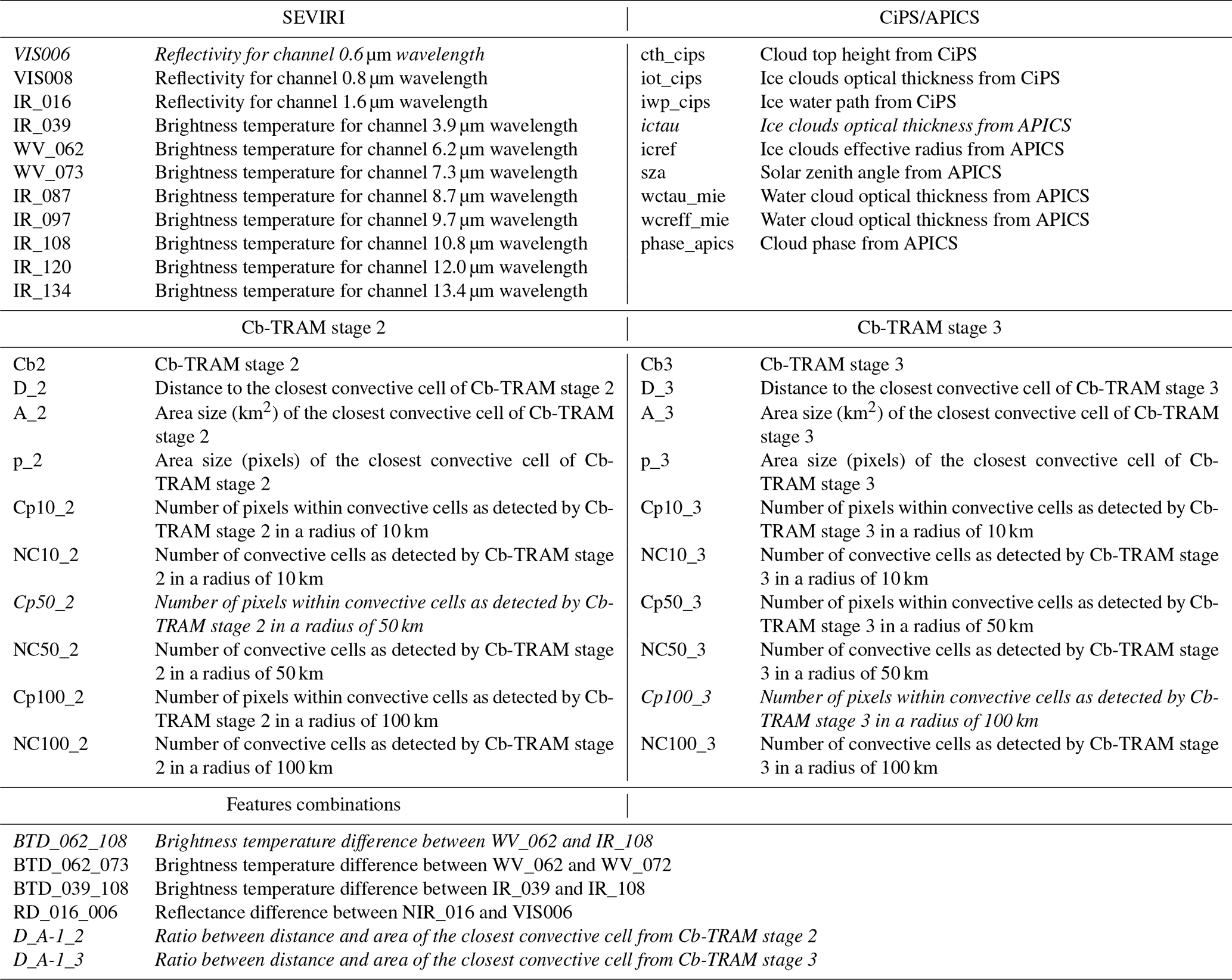
The full list of convection-related metrics with their definitions is presented in Table 2.

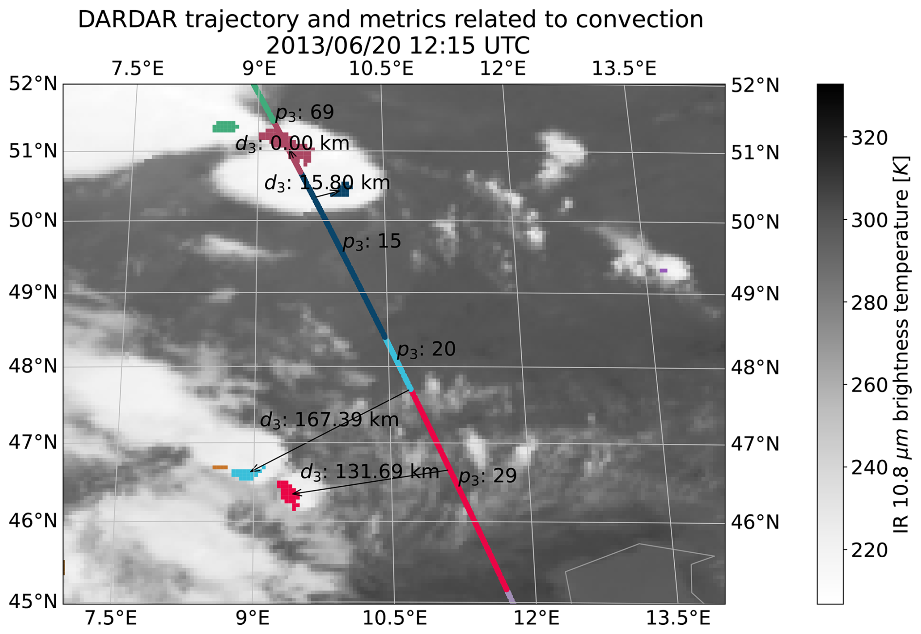
Figure 2 Demonstration of the convection-related variables integrated in the DARDAR dataset. The DARDAR trajectory is color-coded according to the closest convective cell detected. For each color portion in the trajectory, the closest pixel to the respective closest convective cell is indicated by the starting points of the arrows. The distance d₃ is displayed along the arrow. p₃ indicates the areal extent in terms of pixels of the convective cell with the corresponding color. The complete list of convection-related metrics with their definitions is presented in Table 2.

Table 2 Candidate input predictors for the potential ICI detection. Chosen input predictors for the random forest are highlighted in italics.

2.4 Lufthansa ICI database

The Lufthansa ICI database comprises 100 pilot-reported ICI events selected manually based on in situ measured total air temperature anomalies (Kalinka et al., 2023). Figure 3 displays the database's geographical distribution. The database is also important to get an indication of the seasonal occurrence of these events, with a special focus devoted to the European continent. We focused on this region because the products that we have used as high ice water content predictors are limited to the upper part of the SEVIRI HRV channel, which remains still over Europe and North Africa. The ICI events distribution agrees with expectations. The majority of them occurred in the Northern Hemisphere summer (JJA). In Europe, two events occurred in autumn (SON) and two in spring (MAM). Therefore, we focus on processing DARDAR trajectories during the summer months to maximize the chance of sampling HIWC conditions in Europe.

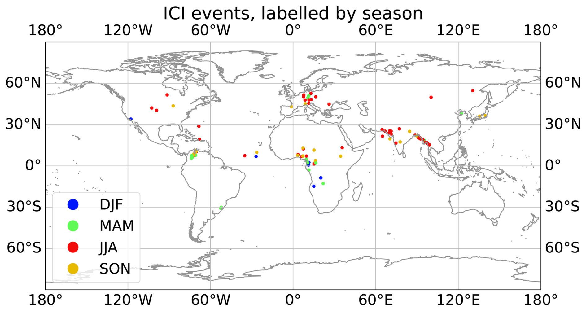
Figure 3 Locations of the Lufthansa ICI events collected in 2016, color-coded according to the season they were recorded.

In Fig. 4, we present the ICI events related to the standard envelope FAA 14 CFR Part 33 Appendix D (Federal Aviation Administration, Department of Transportation, 2023), which depicts where ICI events occur in terms of altitude vs. ambient temperature. Most of the events collected by Lufthansa fall within the specified boundaries, except for three cases. 88 % events occur between 9000 m (29 527 ft) and 13 000 m (42 650 ft). This altitude band, called “cruise levels” hereafter, indicates the portion of the troposphere that is considered when sampling IWC in the cloud profile from active satellite instruments. Furthermore, while testing for multiple cruise level limits (not shown), we observed that the correct detection of HIWC conditions was more likely when these conditions occur at higher altitudes, as observed also by de Laat et al. (2017). We speculate that this is due to passive sensors measuring emitted and reflected radiation in proximity to cloud tops, thus inherently limiting the in-cloud HIWC detection.

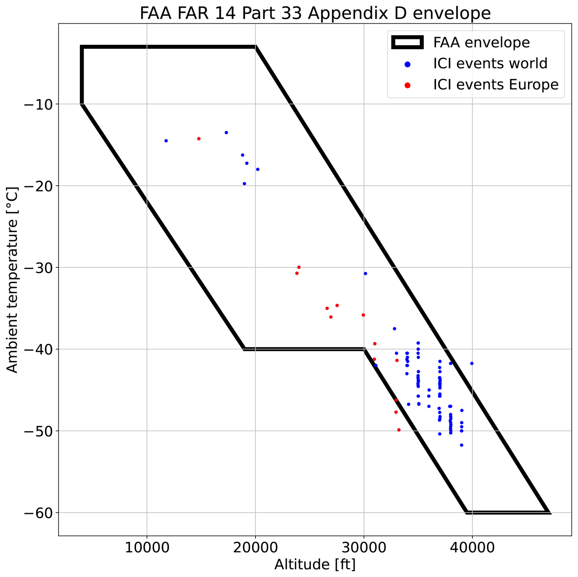
Figure 4 FAA 14 CFR Part 33 Appendix D (Federal Aviation Administration, Department of Transportation, 2023) standard envelope encloses typical air temperature and altitudes found for ICI conditions. The points denote the temperature and altitude associated with the events in the Lufthansa ICI database.

3 ICI retrieval

The core idea behind the ICI retrieval is to combine a broad range of predictors measured by passive instruments on board geostationary satellites (Sect. 2.1) to detect potential ICI events, determined with DARDAR measurements of HIWC conditions. The retrieval, based on a random forest approach, estimates the probability of HIWC conditions. By setting a threshold on the probability of HIWC conditions, one can convert this information to the HIWC binary flag to use it as a deterministic target output variable for the ICI retrieval training and validation. Finally, the ICI retrieval can be applied to geostationary imagery to obtain a probability mask of HIWC conditions.

Random forest classifiers are an ensemble method based on single decision trees. Decision trees divide recursively the predictor space into distinct non-overlapping regions, which are the tree's nodes. The split is aimed at minimizing the output variance within each region. The output probability to predict a certain class is the proportion of that class found in the training dataset for the end nodes, or leaves. The main disadvantage of single trees is that they are very sensitive to the training dataset. Hence, the need for random forests, which reduce the variance by averaging a set of single trees. Because random forests have many hyperparameters that can be tuned by the user, such as the number of trees, the tree depth, and the number of samples allowed in the leaves, it is often necessary to determine them through cross-validation. Cross-validation is a method to estimate the statistical learning method's test error by holding out a subset of the original dataset. K fold cross-validation consists of dividing the dataset into k groups, or folds, of equal size. One fold is treated as the validation set, while the others are used for training. The procedure is repeated for all the k folds, each time considering a different fold for validation. The dataset where the k fold cross-validation is performed is split into training and validation sets. This step is used to tune the hyperparameters, to avoid overfitting and unnecessarily complex models. The cross-validation dataset differs from the test set of unseen observations. This is used to evaluate the actual performance of the model with the chosen hyperparameters.

Figure 5 Illustration of the dendrogram depicting the feature extraction procedure through hierarchical clustering, based on the correlation score among the considered input features. The more correlated the clusters, the shorter the vertical branch extent is. The Ward's distance linkage score represents the correlation-based distance between clusters in our dataset's space. The black horizontal line depicts the suggested level by cross-validation at which the dendrogram should be cut to obtain an optimal number of clusters from which input features can be selected. Different colors depict the clusters obtained according to this cut level. The variables in bold are selected for the final version of the model. The choice is based on permutation importance estimation in Fig. 6.

3.1 Dataset imbalance

Many industry and science-related problems are inherently characterized by data imbalance. Imbalanced datasets in classification problems are those datasets that have output quantities skewed toward a specific class. In the case of binary classification problems, the majority class is over-represented compared to the minority class (Chawla et al., 2004).

The classification of imbalanced datasets significantly challenges the algorithmic approach for several reasons. First, one often wants to predict the minority class. However, the imbalance exposes the classifier to the majority class more frequently during training. For this reason, the minority class can be confused with noise and can be challenging to predict in areas of the data space where both classes overlap (Haixiang et al., 2017). Second, the use of conventional performance metrics, such as accuracy, may reflect the structure of the dataset rather than the classifier's predictive skill. Performance metrics more suitable for imbalanced problems are the Receiver Operating Characteristics (ROC) curve (Chawla et al., 2004) or the Critical Success Index (CSI) (e.g. de Laat et al., 2017). When correcting for the majority and minority class proportion, the ratio between the minority and majority class can be set freely depending on the application, and it is not necessary to exactly balance the two classes (Haixiang et al., 2017).

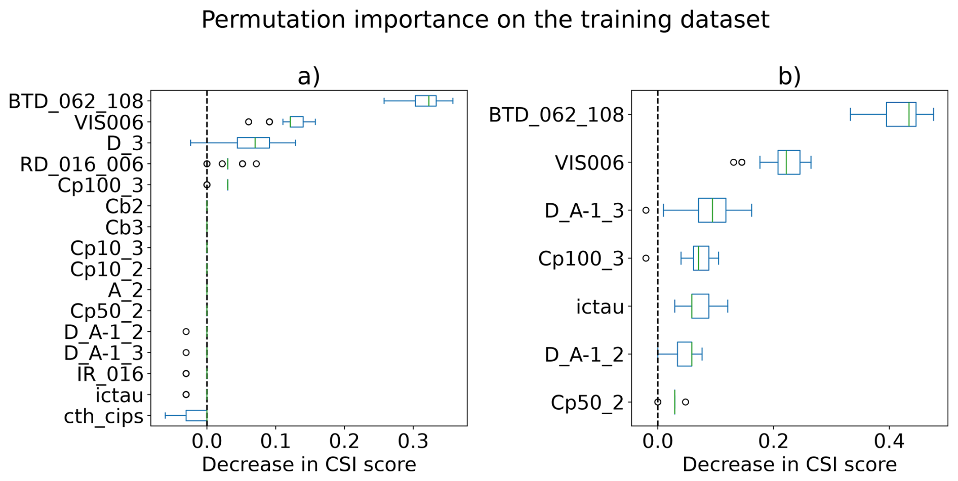
Figure 6 The permutation importance of a variable represents the decrease of the model's performance score (CSI) achieved when that variable is shuffled randomly with respect to the output target. (a) shows the permutation importance of 16 input variables achieved during training applied to four out of five folds in one instance of cross-validation. Similarly, (b) shows the permutation importance of the manually selected input features on an example of a training instance during cross-validation. The box plots depict the distribution obtained when shuffling the variable 50 times randomly. In each box, the green line depicts the median of the distribution, the blue box depicts the interquartile range (IQR), delimited by the 25th and 75th percentiles (first quartile, Q1 and third quartile, Q3, respectively), and the whiskers spread to the last data point within Q1 − 1.5 IQR and Q3 + 1.5 IQR. Any data point beyond the whiskers is shown as an outlier with a white dot.

Table 1 showcases the imbalance between HIWC and no-HIWC sampled pixels by DARDAR. Given the large number of no-HIWC pixels, we undersample the original DARDAR dataset. This has a two-fold effect: first, undersampling a large training dataset is more computationally efficient (Chawla et al., 2004). Second, carefully choosing the undersampling technique reduces the correlation between samples. Indeed, samples of the same DARDAR trajectory correlate in time and space. Correlated samples may induce a bias in the training and validation procedure. This problem is also mentioned by Haggerty et al. (2020) in the case of aircraft measurements.

The undersampling is performed as follows:

• for the DARDAR trajectories with at least one HIWC sample, all HIWC samples belonging to that trajectory are taken, maintaining a buffer distance of 10 pixels if multiple consecutive pixels are flagged with HIWC;

• for DARDAR trajectories with no HIWC samples, pixels are sampled randomly among binned ranges of brightness temperature in the 10.8 µm channel, cloud optical thickness, and distance to the closest convective cells to cover a variety of HIWC-free conditions sufficiently.

Undersampling produces a new proportion between the classes depicted in Table 1. Although still imbalanced, a more aggressive undersampling was tested but led to undermining the subsequent model learning due to a too strong reduction of the variability of the majority class and, consequently, its representativeness. Finally, the test dataset contains five not undersampled DARDAR trajectories with at least one HIWC pixel.

3.2 Feature selection and random forest algorithm

The full list of input features considered for the potential ICI detection from SEVIRI is shown in Table 2.

The high-dimensional dataset produced when considering all the input predictors induces the so-called “curse of dimensionality” (James et al., 2021). In such cases, irrelevant or redundant predictors may act as noise and may lead to inefficient and inaccurate learning (Chawla et al., 2004). Furthermore, a high number of features can affect the variance-bias trade-off characterizing statistical learning methods: having a large set of features, even if relevant, may lead to an increase of variance that eventually outweighs the bias reduction produced by a more sophisticated model (James et al., 2021).

In our case, many features considered for the learning process are correlated by design, e.g. the variables originating from the same geostationary retrieval or the area of the convective cells expressed in km² and in the number of pixels. These redundant features may act as noisy features and exacerbate the curse of dimensionality. Therefore, a feature selection approach is chosen to reduce the dimensionality of the input data. This approach selects a subset of input features that optimizes the classifier's performance.

First, to perform the feature selection, the input features' correlation coefficient is determined for all the possible permutations of input predictor couples. This allows building a correlation matrix converted into a correlation-based distance (Ward's distance linkage score on the vertical axis of Fig. 5), which is considered a dissimilarity measure between the predictors. This distance creates a fictitious space within which input predictors are represented as data points. Then, the input feature subsets are obtained using hierarchical clustering, which is a bottom-up approach that assigns, as the first step, one cluster to each sample in the dataset's space. In our case, the samples are the input predictors. Eventually, it progressively identifies affine clusters and merges them until all sampled points end up in a single cluster, corresponding to the full dataset (James et al., 2021).

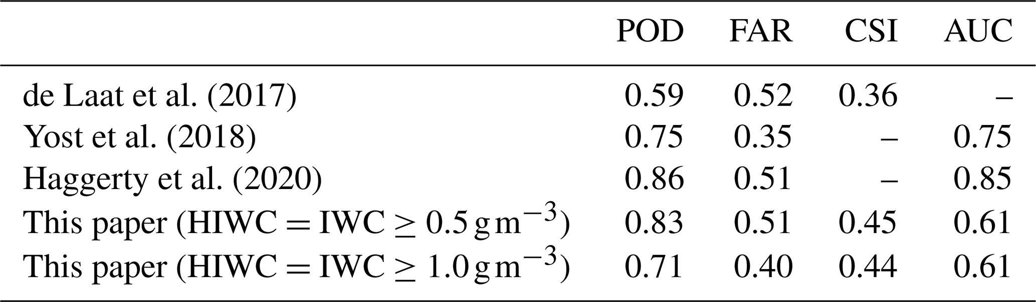
de Laat et al. (2017)Yost et al. (2018)Haggerty et al. (2020)

Table 3 Performance metrics comparison of the random forest ICI retrieval presented in this paper vs. the previously developed ICI retrievals. Although the training and verification techniques differ, as well as the retrieval's applicability, these results are reported to place this work in the current research context. The metrics shown correspond to the median value of POD, FAR, CSI, and AUC found in Fig. 8. Both $\text{HIWC}=\text{IWC}\ge \mathrm{0.5}\mathrm{g}{\mathrm{m}}^{-\mathrm{3}}$ and $\text{HIWC}=\text{IWC}\ge \mathrm{1.0}\mathrm{g}{\mathrm{m}}^{-\mathrm{3}}$ performance are referred to the model trained as described in Sect. 3. The $\ge \mathrm{1.0}\mathrm{g}{\mathrm{m}}^{-\mathrm{3}}$ results in a lower occurrence of HIWC, thus this version is adapted with a HIWC probability threshold of 0.7. (Yost et al., 2018) and (Haggerty et al., 2020) developed both daytime and nighttime retrievals, but the metrics reported here refer to daytime only.

The dendrogram depicts the bottom-up clustering, starting with a cluster containing all the input features at the top and then progressively splitting into multiple branches, each representing one cluster. Feature selection can be implemented by cutting the dendrogram at a certain level of the distance score on the vertical axis. In our case, the cutting level is initially determined through cross-validation to produce 16 clusters. The cutting level line crosses the dendrogram's branches multiple times. Features that can be reached from the same cut point following the branches belong to the same cluster. Features belonging to the same cluster are redundant in the sense that they give access to similar information to the statistical model through the learning process. Therefore, one feature per cluster is selected to obtain a subset of features suitable for learning with imbalanced data.

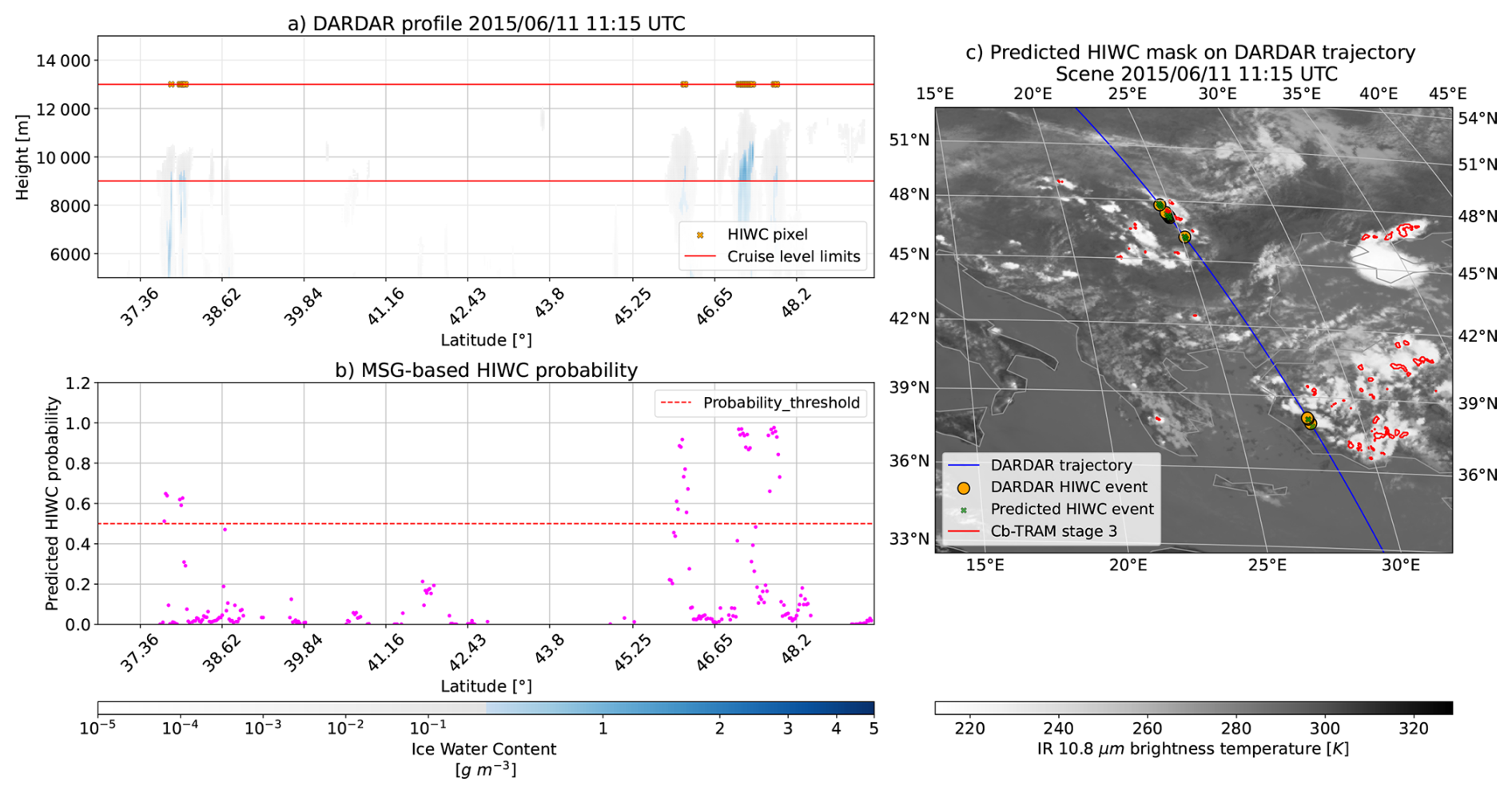
Figure 7 The HIWC conditions retrieval validation based on DARDAR trajectories. (a) shows the IWC cloud cross-section profile with the associated HIWC flags assigned with the criteria described in Sect. 2. (b) depicts the corresponding HIWC probability predicted by the random forest. (c) displays the DARDAR trajectory in the respective MSG image and the prediction of HIWC conditions converted from the probabilistic prediction.

Furthermore, the permutation importance score allows the estimation of the importance of the selected features by hierarchical clustering. This evaluation requires setting a statistical model and a statistical performance metric that one wishes to optimize, which, in our case, are a random forest and the CSI, respectively. The method consists of shuffling the values of each predictor in the dataset to produce a corrupted dataset, which is fitted to the model chosen. The performance score is then compared with the score of the original dataset. The predictors may be correlated if the model maintains an overall constant predictive skill, but no predictor appears to be important according to the permutation importance score estimation. In this case, applying the permutation to one of them does not lead to a significant performance decrease because the model can access the same information via the correlated feature. This behavior can be seen in Fig. 6. In panel (a), the initial choice of 16 input variables reveals that a few features are important according to the permutation score achieved. This is denoted by the boxplot collapsing into a single line, which indicates that all the simulations carried out led to the same decrease in performance score, thus producing no distributions. Few outliers present for some variables, as for example D_A-1_2, D_A-1_3, IR_016, and ictau, indicates that only a minority of simulations led to a change in performance score. In this case, the model performs well during the training, which can be an indication of correlated features. Shrinking to seven variables (panel b) does not hinder the model's performance, but all input features become important. This further suggests that panel (a) contains correlated features. The input features are selected manually based on the achieved permutation importance score obtained in the cross-validation, commonly used predictors in previous ICI detection retrievals, and the physical knowledge of the ICI phenomenon. From the predictors' list in Table 2, BTD_062_108 is selected because it is a proxy for updraft speeds (Bravin et al., 2015; Grzych et al., 2015; Yost et al., 2018), VIS006 and ictau are chosen for their ability to highlight optically thick and highly reflective deep convective clouds, while the convection metrics Cp100_3, D_A-1_3, Cp50_2, D_A-1_2 are selected to account for convective cells density around each pixel and how big and distant the convective cells are from each pixel at different life-cycle stages. It must be noted that the VIS006 and ictau variable choices prevent the retrieval from working in nighttime mode. The selected variables are denoted in italics in Table 2.

A random forest approach is selected to tackle this problem because it is among the most popular approaches to deal with imbalanced classification problems, guarantees interpretability, and can handle large datasets (Haixiang et al., 2017). Finally, the 5-fold cross-validation procedure also led to the random forest hyperparameters choice of 1000 trees inside the forest, 5 minimum allowed samples that can be included in each node at the end of the tree, and a probability threshold of 0.5 to convert from the probabilistic into the deterministic forecast.

4 Retrieval application and validation

4.1 Retrieval performance test through DARDAR profiles

The statistical metrics chosen to assess the retrieval's performance are well established in the atmospheric science literature (Wilks, 2019). Their definitions can be found in Sect. A1.

The retrieval test dataset contains five randomly selected DARDAR trajectories with at least one HIWC pixel. These trajectories are left out of the training and cross-validation procedure. In Fig. 7, we present an example of the DARDAR trajectory used to test the potential ICI detection. Panel (a) shows the cloud's IWC profile where one can see two areas of HIWC conditions: the first, around 37° N, originating from two adjacent deep clouds, and the second, in the proximity of 47° N latitude, composed by a set of three vertically developed clouds that produce three nearby but distinct HIWC areas. Clouds at 37° N are characterized by a notable vertical extent of HIWC conditions with IWC reaching the maximum value of 0.8 g m⁻³ within the cruise levels and by cloud tops extending up to 10 410 m. The clouds composing the system at 47° N have more extended HIWC conditions. The central cell is by far the most active in terms of HIWC, with a peak IWC value of 1.1 g m⁻³ and the cloud top at 11 940 m altitude. The corresponding MSG-based HIWC probability is displayed in panel (b). This is plotted only for icy cloud pixels according to the CiPS mask and it is characterized by a sharp transition from low to high HIWC probabilities. One can also see that the clouds around 37° N have a lower HIWC probability when compared to clouds at 47° N, even though still above the threshold of 0.5. This can be attributed to a relatively higher density of stage 3 convective cells detected by Cb-TRAM near the trajectory.

To assess the overall robustness of the presented approach, the training and subsequent testing are repeated 100 times, each time with another random selection of 5 DARDAR trajectories as test data. The repeated tests generate the distribution in the performance metrics shown in the box plots of Fig. 8. The large variability may suggest the need for further data, as the method seems very sensitive to the training and test datasets used. The median values of POD=0.83, FAR=0.51, CSI=0.45, and AUC=0.61 are similar to previous retrieval performances, depicted in Table 3. For our retrieval, POD is the least spread metric with 75 % of the tests lying above 0.79, denoting a high probability of detecting positive events correctly. On the other hand, FAR spreads over a much larger range, which is also reflected in the CSI and AUC variability. Focusing on the AUC, this metric lags behind when compared to Yost et al. (2018) and Haggerty et al. (2020) retrievals. The model has been tested with $\text{HIWC}=\text{IWC}\ge \mathrm{1.0}\mathrm{g}{\mathrm{m}}^{-\mathrm{3}}$. The original version is used, trained with samples labeled as HIWC if $\text{IWC}\ge \mathrm{0.5}\mathrm{g}{\mathrm{m}}^{-\mathrm{3}}$ and adapted with a higher probability threshold of 0.7, to compensate the lower occurrence of HIWC when those are defined with the higher threshold of 1.0 g m⁻³. Table 3 shows that, in this case, FAR is reduced significantly, at the expenses of a decreased POD. CSI and AUC do not vary compared to the test settings consistent with training settings.

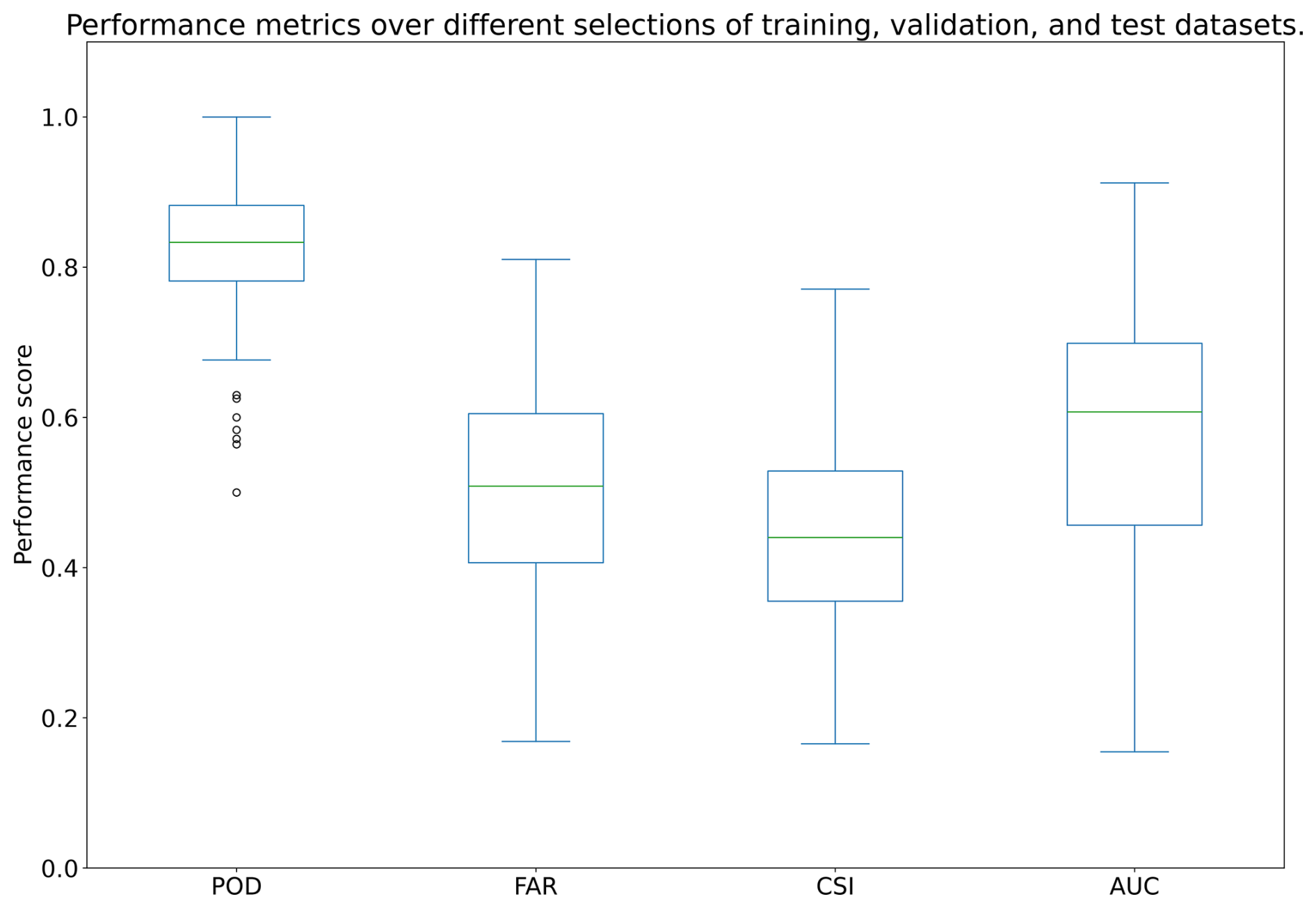
Figure 8 Performance metrics variability in the repeated training and test procedure. The box plots represent the obtained performance scores over 100 iterations. The main central box depicts the interquartile range (IQR), which is the range between the 25th (first quartile, Q1) and 75th percentiles (third quartile, Q3) of the distribution. Whiskers are defined by the last data points lying within Q1 − 1.5 IQR and Q3 + 1.5 IQR. Anything lying outside the whiskers is considered an outlier.

The relatively low AUC in both test settings can be linked to the sharp transition from low to high HIWC probability. The sharp probability transition means that acceptable POD can only be achieved if one allows a substantial FAR, suddenly leading the ROC curve to shift from below to above the chance line and eventually producing a low AUC. This sharp transition of predicted HIWC probability can also be observed in Fig. 10, where the two-dimensional HIWC probability mask is shown.

To explain the high FAR incidence, one can observe Fig. 9. Focusing on the convective system between 33 and 36° N latitude, HIWC conditions within the cruise levels are present in the DARDAR dataset in the southern and northernmost parts of the system. In contrast, the inner parts are characterized by HIWC conditions only below the cruise levels. However, the MSG-based HIWC probability stays above the threshold throughout the horizontal extent of the cloud, though with a small dip in the middle section. This is reflected in panel (c), where HIWC conditions are predicted for the entire cloud rather than just the two extremes, giving rise to a high FAR. de Laat et al. (2017) and Haggerty et al. (2020) also observed a relatively high FAR. Haggerty et al. (2020) concludes that most FAR pixels are associated with HIWC conditions occurring at altitudes different than the ones sampled by the aircraft. This is also the case for Fig. 9. However, in this instance, cruise levels are chosen according to the altitude at which ICI events occur in the Lufthansa ICI database. Nonetheless, the best trade-off to retrieve cloud properties remains challenging to find. Cloud properties vary within the cloud structure, while passive sensors can only detect cloud top characteristics or column-integrated quantities. The HIWC conditions detection presented is compared with previously developed retrievals to put this work in the current research context. However, these retrievals have different characteristics. Namely, this method differs by data sources, input features, clouds' microphysical characteristics retrievals, and detection approaches. Furthermore, our retrieval is tested and validated in the Europe domain, and not globally as in e.g. de Laat et al. (2017).

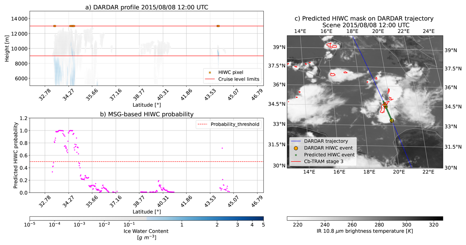
Figure 9 As in Fig. 7 for a different DARDAR trajectory example.

4.2 Lufthansa case studies

The Lufthansa ICI database is presented in Sect. 2.4 and contains 10 case studies in Europe out of the 100 cases available globally. Three events are encountered at night, but nighttime scenes are discarded because of the absence of visible channels and optical thickness data. ICI events are correctly detected by the HIWC mask in four out of the seven remaining daytime scenes.

The criterion for correct detection considers the last available aircraft position, labeled as ICI position, and whether the predicted HIWC probability is larger than our threshold of 0.5. This criterion is applied irrespective of the time difference between the aircraft measurements and the satellite acquisition time, which could be up to 7 min and 30 s. The three scenes in Fig. 10 are a subset of the processed scenes, selected according to the smallest time delta between the aircraft measurement and the satellite acquisition time. Appendix A contains the remaining Lufthansa case studies.

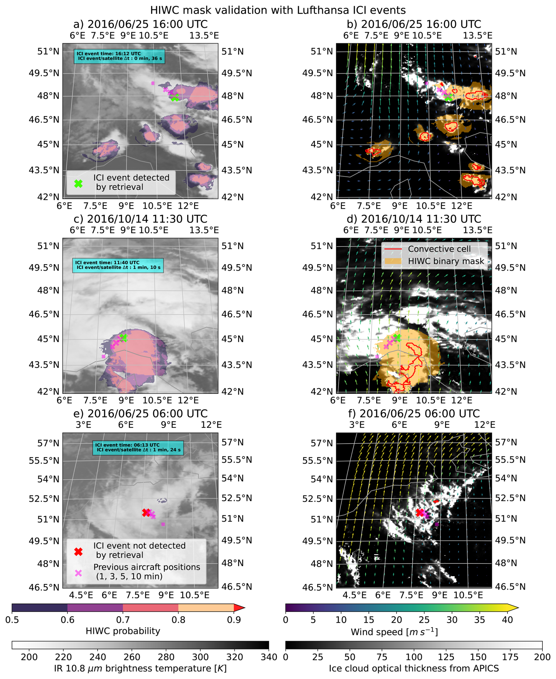
Figure 10 (a), (c), and (e) show the HIWC probability mask with the respective aircraft's positions before and during the in-service ICI events. The ICI event time is shown in the text box with its time delta compared to the actual satellite acquisition time. (b), (d), and (f) show the respective HIWC binary masks, converted using the 0.5 HIWC probability threshold. The mask is combined with Cb-TRAM stage 3 convective cells and horizontal wind field at 300 hPa from ECMWF ERA5 reanalysis data and ice cloud optical thickness from APICS.

In Fig. 10a and c have large areas of HIWC high probability, often exceeding 0.7–0.8. The mask generally has a sharp transition from 0.5 to 0.7 HIWC probability and seldom approaches 1.0 (a few small areas in panel (c). The HIWC mask is almost completely absent in panel (e), with small patches of 0.5 HIWC probability around the Cb-TRAM stage 3 convective cell seen in panel (f). The HIWC binary mask shown in panels (b), (d), and (f) is compared with the detected Cb-TRAM convective cells and the ECMWF ERA5 reanalysis wind field at 300 hPa. The model data in panels (b), (d), and (f) have an hourly resolution; therefore, scenes (b) and (f) have simultaneous satellite images and wind fields, while for scene d), the wind field refers to 11:00 UTC.

The HIWC masks generally differ from the Cb-TRAM convective cells and the ice optical thickness from APICS. The HIWC masks often stay around detected convective cells with high optical thickness and cold cloud tops, highlighting the need for a dedicated HIWC detection product. In particular, it is possible to observe that the masks propagate downstream of the detected convective cells, even though the wind is not used as an input feature. In panel (b), the wind field is relatively weak in correspondence with the biggest HIWC mask patches. The HIWC mask tends to follow the wind field for the convective cells between 45 and 46.5° N latitude, but this behavior is less evident for the big HIWC patch at 48° N latitude. Instead, panel (d) depicts strong wind fields and a large HIWC mask propagating downstream of the main convective cores detected by Cb-TRAM.

From the correctly detected events, airplanes flew inside the HIWC mask before the aircraft's final location, where ICI was reported. This might indicate that aircraft have to fly within ICI conditions for some time to guarantee enough exposure to such conditions for ice to accrete inside the engines. This would also be consistent with one of the failed detections presented in App. A, where the flight flew through the HIWC mask before the final position that falls right outside the mask. For the failed detection in Fig. 10e, we speculate that the HIWC mask is missing due to the absence of large convective cells in panel (f). Although ICI events are almost exclusively attributed to convection in the literature (Grzych, 2010; Bravin et al., 2015), ICI events have also been reported in different conditions, such as within extra-tropical cyclones (Gayet et al., 2012). Panel (f) could suggest that this retrieval would fail when Cb-TRAM cannot detect deep convective cells.

4.3 Nighttime performance

The retrieval is here tested during nighttime. In this scenario, the random forest model does not have access to visible channel information and cloud optical thickness. Furthermore, it has been trained exclusively with day-time samples. Nevertheless, it can access infrared channels and convection related variables.

In night-time mode, we decided to use instrumental values to fill the missing information required by the random forest approach. In Fig. 11, the distribution in the training dataset of VIS006 and ictau for HIWC and no-HIWC is shown. These distributions allowed us to select a bias-free value with which we filled the missing information in nighttime mode. In particular, this bias-free value is selected such that it favors neither HIWC prediction, nor non-HIWC, i.e. the instrumental value should be in a range where HIWC and no-HIWC training samples distributions overlap. The values are set to VIS006=80 % and ictau=50.

Figure 11 (a) VIS006 and (d) ictau samples distributions in the training dataset, for HIWC (orange) and no-HIWC (blue). Negative values in both distributions arise because of the curve smoothing for plot purposes. The real sample locations are visible in (b) and (d).

The significance of this choice is shown in Fig. 12. The mask in panel (a), where we set VIS006=0 % and ictau=0, is absent because the HIWC probability never exceeds 0.5. In panel (b), the bias-free choice of VIS006=80 % and ictau=50 leads to a smooth transition of HIWC probability bewteen areas without detected HIWC and areas where HIWC is detected. Panel (c) displays instead a sharp transition to high HIWC probabilities, as soon as this is detected by overcoming the 0.5 probability threshold. We observe that the constant instrumental values with which we fill missing information modulate the HIWC probability mask significantly. The choice made for panel (b) is the best to achieve realistic results even with missing solar information. This demonstrates the good performance of the model even during nighttime.

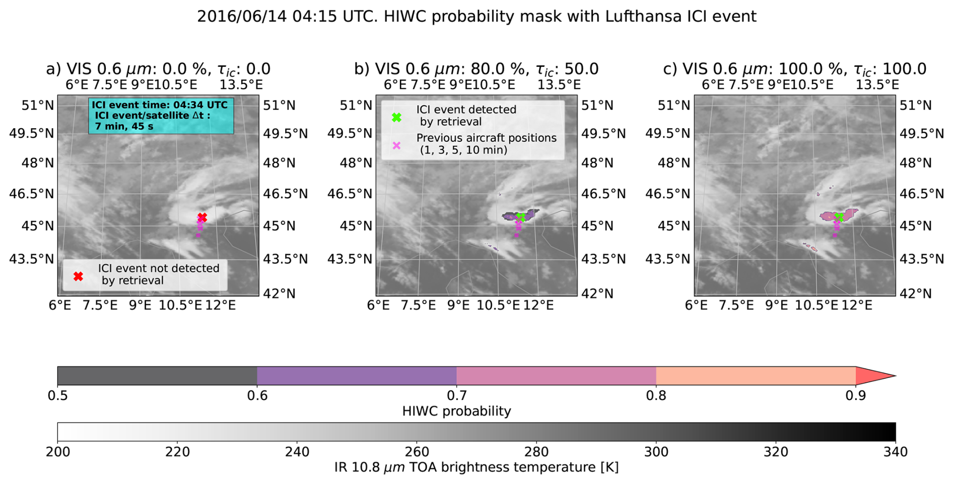
Figure 12 ICI retrieval nighttime mode demonstration example for a Lufthansa ICI event. (a) shows the HIWC mask setting instrumental values that favor no-HIWC prediction (see Fig. 11). (b) depicts the HIWC mask with bias free instrumental values. (c) shows the HIWC mask with instrumental values favoring HIWC predictions.

4.4 Validation with in-situ measurements: HAIC-HIWC II campaign

Finally, the algorithm was validated with a case study of the HIWC-HAIC II flight campaign (Strapp, 2016). However, Cb-TRAM is not available for the tropical regions covered by this campaign (see Sect. 2.1.3). Therefore, to cover this domain, alternative data are retrieved. Deep convective systems are provided by the TOOCAN database (Fiolleau and Roca, 2013, 2019). To prove the adaptability of the method to any equivalent product than the ones presented in the Sect. 2.1, cloud optical thickness was retrieved via the Optimal Cloud Analysis data record (EUMETSAT, 2022). The aforementioned data are displayed in Fig. 13.

Figure 13 Satellite scene for the HAIC-HIWC II campaign case study. We considered flight 23, flying from French Guyana the 26 May 2015. (a) shows the SEVIRI visible channel at 0.6 µm wavelength reflectivity. (b) depicts the cloud optical depth from Optimal Cloud Analysis (EUMETSAT, 2022) and deep convective cells from the TOOCAN database (Fiolleau and Roca, 2019).

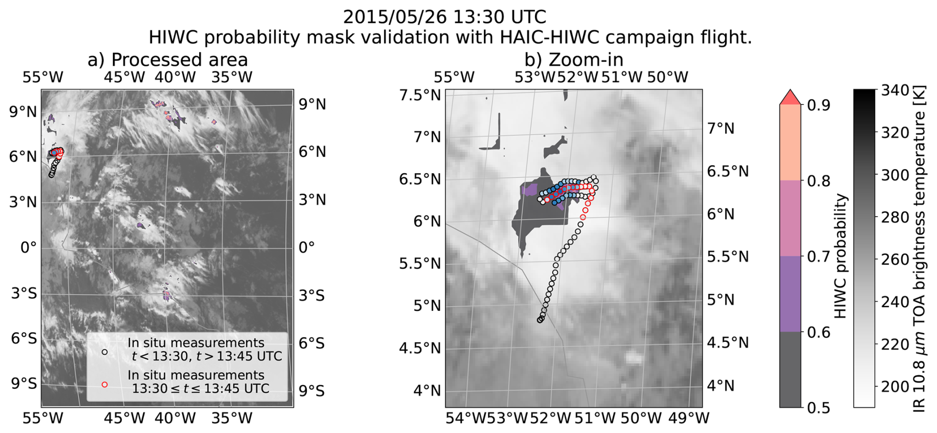
Figure 14 HIWC mask validation with flight 23 of the HAIC-HIWC II flight campaign. The flight crossed a HIWC region ($\text{IWC}\ge \mathrm{0.5}\mathrm{g}{\mathrm{m}}^{-\mathrm{3}}$) from 13:37 to 13:45 UTC peaking at 13:41 UTC with $\text{IWC}=\mathrm{3.3}\mathrm{g}{\mathrm{m}}^{-\mathrm{3}}$. HIWC measurements are depicted in blue shades, while no-HIWC are shown in grey shades. Markers with red borders depict the flight position within the satellite scanning times. Flight waypoints are corrected for parallax effect, shifted to the corresponding satellite grid coordinates.

Figure 14 shows the corresponding computed HIWC mask. Although convection is widespread throughout the domain in Fig. 13b, the HIWC mask is relatively limited in extent in Fig. 14a. It features HIWC probabilities higher than 0.9 for convective cells around 40° W and 9° N, and 40° W and 3° S, while HIWC probabilities closer to the flight (52° W and 6° N) are relatively lower, peaking at 0.7. Panel (b) shows a good agreement between the measured HIWC and the HIWC probability mask. $\text{IWC}\ge \mathrm{0.5}\mathrm{g}{\mathrm{m}}^{-\mathrm{3}}$ sampled points mostly fall within the mask, whose values increase together with the measured IWC. The retrieval shows promising results even outside the domain where it was trained, and using input data equivalent to the ones discussed in Fig. 2.1. Given the results obtained with this case study, we speculate that only little calibration would be required to adapt the retrieval to input parameters coming from different data sources.

5 Conclusions and outlook

In this study, our goal is to assess the feasibility of a detection retrieval for potential ICI conditions, based exclusively on remote sensing data and a random forest approach as a machine learning technique. A combination of passive remote sensing measurements from geostationary satellites is used to detect areas with HIWC conditions at passenger aircraft cruise levels. These conditions are chosen as an indicator for potential ICI formation. Cruise levels are considered because, even if ICI events are possible during the ascent and descent of an aircraft, passive remote sensing platforms are more sensitive to cloud tops and column-integrated quantities. For the training phase, HIWC conditions are located from active measurements of IWC from polar-orbiting satellites, i.e. the DARDAR dataset, which is taken as ground truth. The results obtained by testing this approach with DARDAR trajectories lead to median values of the performance metrics POD=0.83, FAR=0.51, CSI=0.45, and AUC=0.61. This method outperforms the approach presented by de Laat et al. (2017), who validated their algorithm globally with DARDAR data, and it achieved comparable results to Haggerty et al. (2020). However, Haggerty et al. (2020) used multiple input sources, such as ground-based weather radar and numerical weather prediction, in addition to geostationary satellite images. In this study, we used only the latter.

The validation of the retrieval is also supported by a database of ICI case studies reported by Lufthansa during operational conditions. The retrieval correctly detects four out of seven events, assuming a correct detection whenever the aircraft's final position is within the HIWC mask. From the observation of the case study examples, the HIWC mask surrounds convective cells in areas with optically thick clouds and glaciated cloud tops. Moreover, the mask often follows the wind field downstream of convective cells, which is physically reasonable but not necessarily expected, as the wind field is not explicitly included as an input feature. The failed HIWC conditions detection in the scene without convective cells highlights the importance of convection signatures to obtain a high probability HIWC conditions signal. This is coherent with past literature, where deep convection and ICI events are often found to be correlated. However, in different conditions, such as in extra-tropical cyclones, the failed detection example indicates that the retrieval could have less chance to detect HIWC conditions when there is no deep convection.

The retrieval demonstration use during nighttime and the comparison with in-situ measurements from the HAIC-HIWC campaign show the adaptability of this algorithm to different conditions, accepting missing optical information during nighttime, and different data sources for convection and cloud microphysical properties.

Integrating the ICI retrieval with cloud microphysical properties retrievals would enable scientific studies about the possible ice formation pathways during ICI events, especially exploiting the temporal resolution of geostationary satellites, as these are not yet understood (Leroy et al., 2017). For example, one could correlate potential ICI areas with retrieved ice particles' effective radius and updraft speeds that can be either taken from reanalysis data or satellite images. A fully operational ICI detection product would require additional development, as it uses visible channels and optical thickness that prevent this retrieval from detecting HIWC conditions at night. Future development would include a more flexible way to select input predictors according to availability. Furthermore, the training dataset could be enlarged, considering the overlap between MSG-3 and DARDAR between 2013–2017. To conclude, the retrieval shows promising performance in detecting potential ICI conditions, using exclusively geostationary satellite imagery as input. This would allow a flexible extension to other geostationary satellite platforms, and its operational implementation would enable airlines to avoid HIWC conditions to mitigate ICI effects on the fleet.

Appendix A:  

A1 Validation metrics

The metrics chosen to assess the retrieval's performance follow the ICI detection retrievals literature (de Laat et al., 2017; Yost et al., 2018; Haggerty et al., 2020) to enable comparison:

• the probability of detection (POD) is defined as the number of correctly predicted positive events (true positives, TP) over actual positive events (TP+FN, where FN stands for false negatives)

  $$\begin{array}{}\text{(A1)}& {\displaystyle }{\displaystyle }\text{POD}={\displaystyle \frac{\text{TP}}{\text{TP}+\text{FN}}}\end{array}$$

• the false alarm rate (FAR) is defined as the ratio between the falsely predicted positive events (false positive, FP) to all predicted positive events (FP+TP):

  $$\begin{array}{}\text{(A2)}& {\displaystyle }{\displaystyle }\text{FAR}={\displaystyle \frac{\text{FP}}{\text{FP}+\text{TP}}}\end{array}$$

• the critical success index (CSI) is an index that balances POD and FAR. It is defined as:

  $$\begin{array}{}\text{(A3)}& {\displaystyle }{\displaystyle }\text{CSI}={\displaystyle \frac{\text{TP}}{\text{TP}+\text{FN}+\text{FP}}}\end{array}$$

• the ROC curve is used to display the variation of two performance metrics simultaneously. They are the POD and the FAR. The ROC curve is useful for classifiers because it explores every possible probability threshold to convert probabilistic into deterministic forecasts. In this way, different classifiers can be compared, no matter the chosen threshold. The chance line is depicted as a diagonal. The model lacks predictive skill if the ROC tends to the chance line. Ideally, the ROC should be a step function. The area under the curve, AUC, measures the overall performance of a classifier across multiple probability thresholds. The chance line has an AUC of 0.5, while an ideal ROC curve approaches 1.0 AUC (James et al., 2021).

A2 Lufthansa case studies

The Lufthansa ICI cases not discussed in the paper are reported here for completeness. Figures A1–A4 are daytime cases. Figure A5 is a nighttime case.

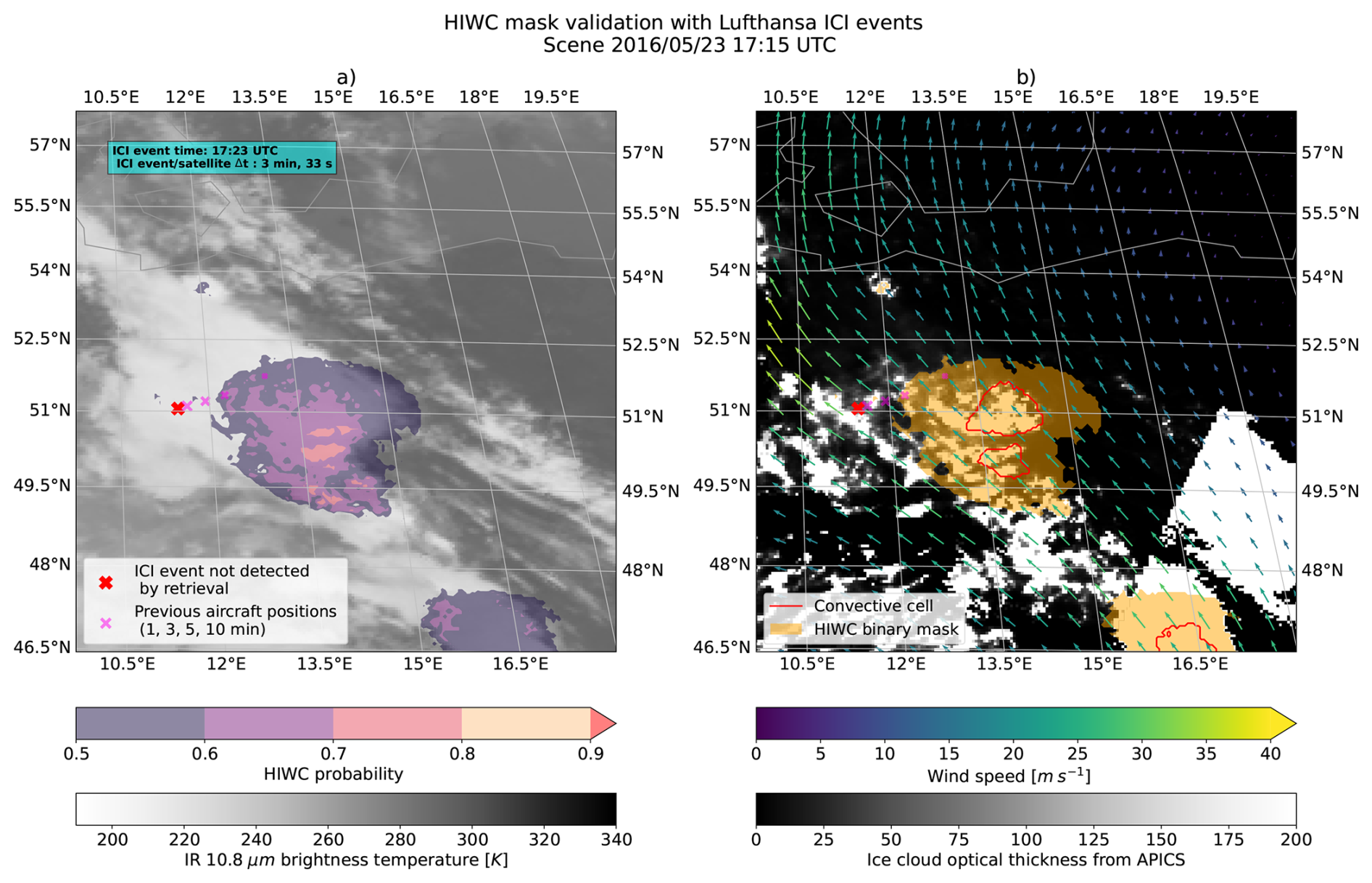
Figure A1 As in Fig. 10a and b for additional Lufthansa ICI case studies.

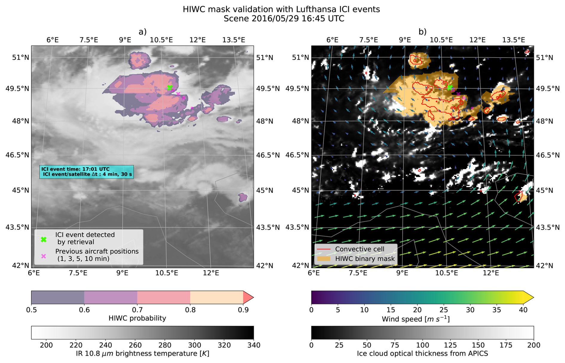
Figure A2 As in Fig. 10a and b for additional Lufthansa ICI case studies.

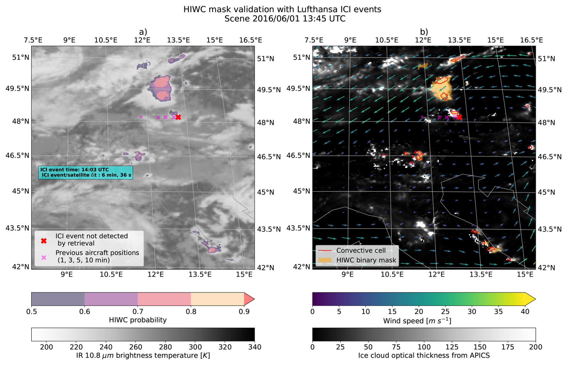
Figure A3 As in Fig. 10a and b for additional Lufthansa ICI case studies.

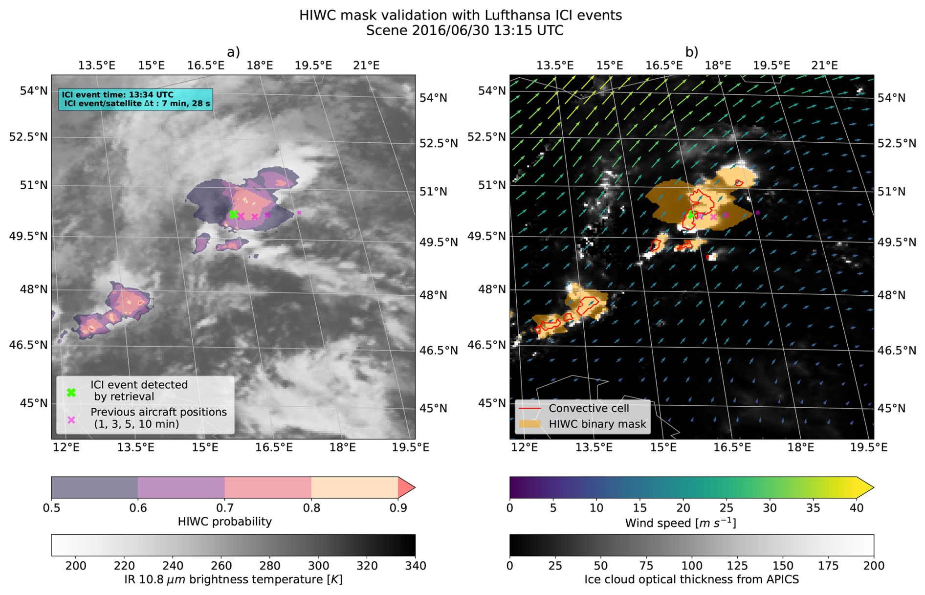
Figure A4 As in Fig. 10a and b for additional Lufthansa ICI case studies.

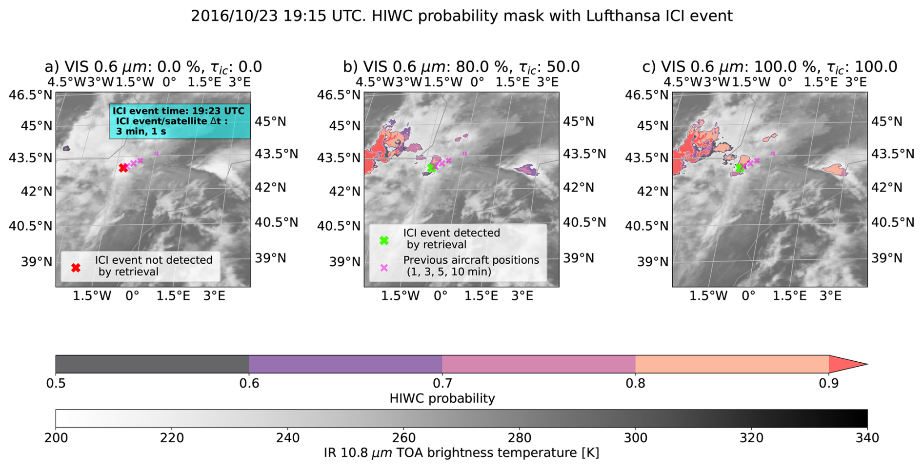
Figure A5 As in Fig. 12 for additional Lufthansa ICI case studies.

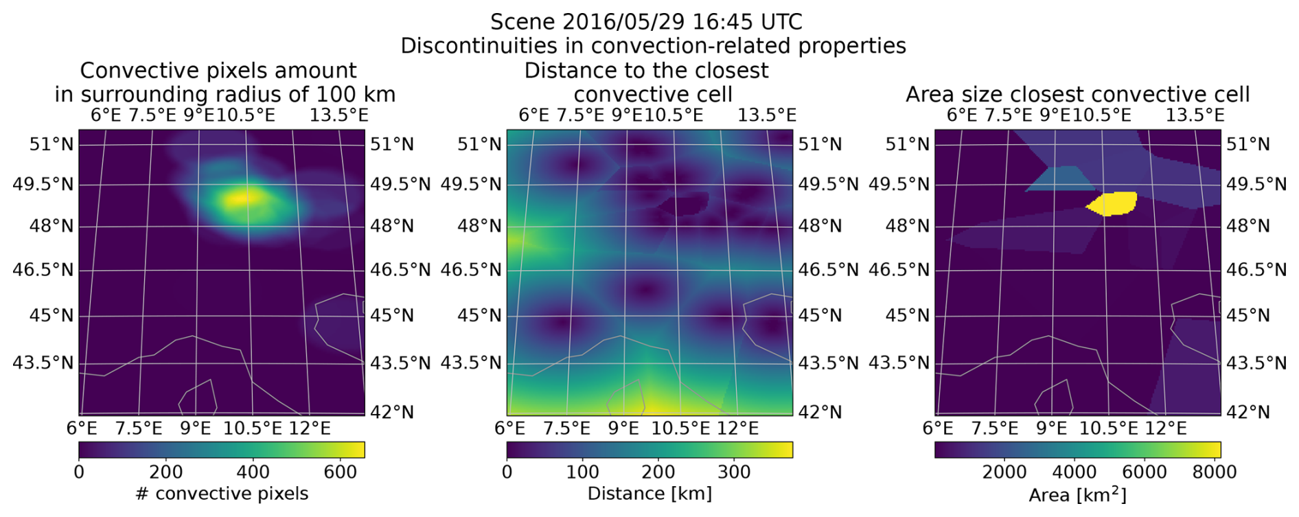
Figure A6 Convection related metrics for the Lufthansa ICI case of Fig. A2 associated with discontinuities.

Figure A7 As Fig. 12, where the nighttime instrumental value approach was applied to a daytime scene, to verify its effect where cloud optical properties would be otherwise available.

A3 HIWC mask discontinuities

Some HIWC probability masks display a discontinuity, as in Figs. A2 and A3. Those discontinuities may be explained with the convection related metrics. Those metrics, such as the distance to the closest convective cell and the areas of the closest convective cell, present such discontinuities, as in Fig. A6. Convective pixels in the surrounding radius of 100 km introduces rounded discontinuities, as in panel (a), while distance and area extent of the closest convective cells introduce linear discontinuities, as in panel (b) and (c). Those discontinuities may be further emphasized by the random forest approach, which does not enforce smooth outputs, but only takes the majority vote from single decision trees. We speculate that the discontinuities might be more pronounced when the other supporting input features, such as visible channels and optical thickness, lie in a region where the split between HIWC and no-HIWC is not clear (see Fig. 11). Thus, this artifact might be more pronounced during nighttime, though this evidence was not found in Lufthansa ICI cases in Figs. 12 and A5. However, this statement is supported by Fig. A7, where the nighttime demonstration approach (Fig. 12) was applied to a daytime scene (Fig. 10a). There, the rounded artifacts due to distance-related convection metrics are emphasized by the artificial unavailability of solar channels information that we introduced as demonstration.

A4 HAIC-HIWC II flight campaign additional case study

Figures A8 and A9 shows an additional case study of the HAIC-HIWC flight campaign. In this case, a HIWC probability mask higher than 0.5 is close to the flight, and it overlaps with its trajectory only where highest IWC is measured.

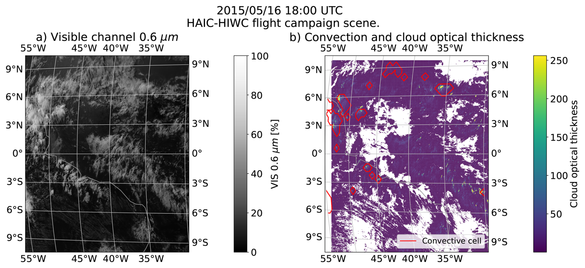
Figure A8 As in Fig. 13 for flight 15 of the HAIC-HIWC II flight campaign.

Figure A9 As in Fig. 14 for flight 15 of the HAIC-HIWC II flight campaign. The flight stayed in a HIWC region during the satellite scan nominal times (18:00–18:15 UTC), with a IWC maximum value of 2.93 g m⁻³ and a median of 1.10 g m⁻³.