Quality assessment of the AC SAF GOME-2 gridded ozone profile data records

One of the objectives of the Atmospheric Composition SAF (AC SAF) is to produce satellite-derived monthly mean data records that are valuable for operational, scientific, and other applications. One of these data records is the gridded global GOME-2A/B/C ozone profile data set presented in this paper. This data record covers the period 2007–2024 and consists of ozone partial columns on a 0.25°×0.25° grid with 40 vertical layers, with the associated (averaged) averaging kernel and the a priori needed to use the data in other applications. This paper presents the GOME-2 instrument, the (level-2) ozone profile retrieval method and the subsequent gridding procedure used to generate the level-3 product. We discuss the methodology for averaging AKs in latitude bands and demonstrate that the principal structural features are preserved. We provide a description of the balloon sounding, lidar, FTIR and microwave radiometers validation data and methods, and then perform a quality assessment of the gridded ozone profile product through comparison with these independent data sources for the tropics, mid-latitude and polar latitude bands for four vertical regions: the Troposphere, the UTLS and the Lower and Upper Stratosphere. Detailed analyses of absolute and relative differences are provided for each region and height range. The results demonstrate a high level of consistency across the three GOME-2 instruments (with GOME-2A used only up to 2018). In the troposphere, all three sensors tend to slightly overestimate ozone, with absolute differences of roughly +1 to +3 Dobson Units (DU) in mid-latitudes and up to +7.5 DU in the tropics for Metop-C. In the more variable UTLS altitude region, the absolute differences range between −2.5 and 5 DU. In the lower stratosphere, all sensors show a small negative bias, typically between −3 and −7 DU (relative difference ≈−3 % to −7 %), corresponding to a modest underestimation of ozone concentrations. In the upper stratosphere, biases are minimal across all sensors, with absolute difference values, close to zero (−0.1 to −0.4 DU) and low variability. These findings underscore the reliability of the GOME-2 constellation for long-term ozone analyses and the potential for merged multi-sensor time series without significant inter-calibration artifacts suitable for climate and atmospheric research.

1 Introduction

Monitoring atmospheric composition is essential due to several human-induced changes in the atmosphere, such as global warming, stratospheric ozone depletion, increased ultraviolet radiation, and air pollution (IPCC, 2023; WMO, 2018; Burrows et al., 2011). In addition, such monitoring enables timely responses to natural hazards and provides the scientific basis for evaluating the effectiveness of international agreements, such as the 1987 Montreal Protocol and its amendments (WMO, 2018).

The Montreal Protocol, implemented in 1989, has been instrumental in reducing the atmospheric concentrations of ozone-depleting substances. As a result, the ozone layer is on a path to recovery (Chippenfield and Bekki, 2024; Solomon et al., 2016). Recent assessments indicate that total column ozone is expected to return to 1980 levels by around 2040 for the near-global average (60° S–60° N), around 2045 for the Arctic, and around 2066 for the Antarctic (WMO, 2022).

However, recovery is not uniform across all regions and altitudes. While ozone in the upper stratosphere has increased significantly – by approximately 1 %–3 % per decade since 2000 (Steinbrecht et al., 2017) – this increase is most pronounced in the mid-latitudes of both hemispheres (Godin-Beekmann et al., 2022). In contrast, the lower stratosphere, particularly in the tropics and mid-latitudes, has not shown clear signs of recovery (Bognar et al., 2022). The increase in upper stratospheric ozone is mainly driven by two factors: the decline in stratospheric chlorine loading following the implementation of the Montreal Protocol and the cooling of the upper stratosphere, which slows the ozone-destroying catalytic cycles and enhances the production of ozone through three-body molecular recombination (Steinbrecht et al., 2025). This vertical and regional discrepancy highlights the importance of sustained, detailed observations of ozone profiles in the stratosphere (WMO, 2018). In addition, tropospheric ozone is of particular importance due to its adverse impacts on air quality, human health, and ecosystems, as well as its contribution to radiative forcing and climate change (IPCC, 2023; Monks et al., 2015). Tropospheric ozone is a secondary pollutant formed through complex photochemical reactions involving nitrogen oxides and volatile organic compounds, and its concentrations are strongly influenced by anthropogenic emissions and large-scale transport processes (Donzelli and Suarez-Varela, 2024; Monks et al., 2015). Satellite-based measurements are central to global ozone monitoring efforts, providing consistent, long-term, and spatially comprehensive data records (Burrows et al., 2011; Xu, 2024). In particular, the Global Ozone Monitoring Experiment (GOME) and its successor GOME-2, flown on board the Metop satellite series, have provided continuous global ozone observations for more than two decades, forming a key component of long-term ozone monitoring and climate data records (Munro et al., 2016; Callies et al., 2000).

This study focuses on the gridded ozone profile products, generated within the framework of the EUMETSAT Atmospheric Composition Satellite Application Facility (AC SAF). These data records are retrieved from measurements of the Global Ozone Monitoring Experiment-2 (GOME-2) instruments onboard the Metop-A, Metop-B, and Metop-C satellites (launched in 2006, 2012 and 2019 respectively). Together, these platforms provide a multi-decadal dataset suitable for long-term assessments.

High-quality ozone profile records are essential for reliable trend detection and are expected to contribute to global assessments such as the World Meteorological Organization (WMO) Scientific Assessment of Ozone Depletion. Therefore, a rigorous validation of the GOME-2 gridded ozone profile data records is required to quantify their accuracy, stability, and suitability for scientific and policy-relevant applications.

In recent years, satellite-based instrument time series of the GOME-type (including GOME-2) have been central to the construction of long-term harmonized ozone profile and tropospheric ozone datasets. Coldewey-Egbers et al. (2025) present the GOP-ECV record, spanning 1995 to 2021, which merges nadir ultra violet (UV) and visible (VIS) measurements from GOME, SCIAMACHY, OMI and GOME-2 into monthly mean partial columns (19 layers, surface to 80 km) on a 5°×5° grid by carefully harmonizing inter-sensor differences and aligning with the GOME-type Total Ozone Essential Climate Variable (GTO-ECV) total-ozone record. Within the European Space Agency (ESA) Climate Change Initiative (CCI) framework, ozone profile retrievals from GOME-2 measurements have also been developed, most notably by the Rutherford Appleton Laboratory (RAL), contributing to the ESA Ozone CCI Climate Data Record (Pope et al., 2023; Sofieva et al., 2023; Ozone CCI, 2010). Although Ozone CCI products mainly aim to construct a homogenized climate data record using multiple sensors and retrieval algorithms, the AC SAF GOME-2 gridded ozone profile products addressed in this study are generated within an operational framework with a strong focus on near-real-time processing, long-term stability, and continuity for user-driven applications. Therefore, both efforts are complementary and jointly contribute to the comprehensive use of GOME-2 measurements for atmospheric ozone monitoring. Arosio et al. (2025) provide an inter-comparison study between existing tropospheric ozone-column datasets derived from combined nadir- and limb-observations, assessing consistency, bias and trend detectability. Keppens et al. (2025) further address the harmonization challenge by combining sixteen tropospheric-ozone satellite records (including GOME-2-derived products) to strengthen confidence in tropospheric ozone time-series and their long-term behavior. Regional studies such as Gaudel et al. (2024) exploit satellite records (including IASI/GOME-2) and in situ profiles to quantify tropical tropospheric ozone trends and regional burdens, while Okamoto et al. (2024) apply a multi spectral IASI + GOME-2 approach over the tropical Atlantic together with aircraft data to discern natural (biomass burning, stratosphere-troposphere exchange) versus anthropogenic influences on tropospheric ozone variability.

Collectively, these works demonstrate that GOME-2 and related sensors now underpin robust ozone-profile and tropospheric-ozone time-series, enabling assessments of spatial distribution, long-term trends and attribution of ozone changes. This paper presents a comprehensive quality assessment of the monthly mean gridded GOME-2A/B/C ozone profile data records. Validation is based on intercomparisons with independent ground-based measurements: ozone sondes, lidar, Fourier transform infrared (FTIR) and microwave radiometers (MWR). The focus is on characterizing the performance of the data products in different atmospheric regions (troposphere, Upper Troposphere/Lower Statosphere interface (UTLS) lower, and upper stratosphere) and over various latitudinal bands, using monthly averaged profiles to evaluate the long-term consistency and bias structure of the dataset.

2 Ozone profiles from GOME-2

2.1 The GOME-2 instrument

The Global Ozone Monitoring Experiment 2 (GOME-2) are a series of nadir viewing instruments mounted on the Metop satellite series. These instruments fly in a polar orbit around the Earth and have an equator overpass time around 09:30 local solar time. The instrument uses back scattered light from the Sun in the UV-VIS spectral region (240–790 nm). The nominal swath width is 1920 km on the Earths surface with 24 pixels in the forward scanning direction of 80×40 km² (cross track × along track). With the (nominal) wide swath width, global coverage can be achieved in 2 d.

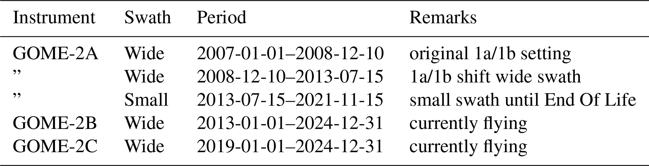
In Table 1 the measurement modes and time periods included in this study are given. The GOME-2A instrument has gone through a number of modes. In December of 2008 the wavelength separation of band-1a/band-1b was shifted from 300 to 283 nm, resulting in stratospheric information with smaller footprints. In mid-July 2013, the swath width was changed from the nominal 1920 to 960 km, which remained until the End of Life de-orbit and shut down of the Metop-A platform in 2021. GOME-2B and GOME-2C have run in the same wide configuration since they were launched.

Table 1 Measurement modes for GOME-2A/B/C.

2.2 Vertical ozone profile retrieval

While the details of the ozone profile retrieval algorithm used to produce the ozone data are given in the Algorithm Theoretical Baseline Document (ATBD) of the Near Real Time (NRT), Offline and Data Record Vertical Ozone Profile and Tropospheric Ozone Column Products (Tuinder et al., 2022), we will provide a description of the relevant aspects of the algorithm below.

The Ozone Profile Retrieval Algorithm (Opera) retrieves vertical ozone profiles from GOME-2 data using the 265–330 nm (UV-VIS) spectral range from the Main Science Channels in band-1a, 1b and 2b. Because of the longer integration time, band-1a is used across multiple smaller band-1b/2b measurements.

The retrieved information consists of a vertical ozone profile of 40 ozone partial column values (in DU) on a fixed pressure grid from the surface to 0.001 hPa, a fitted albedo value (either surface albedo or cloud albedo) and an additional offset to correct for a systematic bias in band-1a (possibly a result of stray light or signal leakage) (Tuinder et al., 2022). The fixed pressure grid is adjusted to the surface height and, in case of clouds, to the cloud top height.

The LIDORT-A radiative transfer model (Spurr et al., 2008) is used in combination with a polarization correction. For the inversion we use Optimal Estimation (Rodgers, 2000), iteratively reaching a converged state of the atmosphere.

Based on the GOME-2 measurement alone, the ozone profile is under-defined, and therefore an a priori ozone profile climatology is used (resolved in latitude bands and months) (McPeters and Labow, 2012).

The (initial) surface albedo comes from the GOME-2 version 3 Directional Lambertian-Equivalent Reflectivity (DLER) database (see Tilstra et al., 2017, 2021). The initial cloud albedo is set to 0.8.

Spectral spikes, such as those caused by highly energetic particles common over the South Atlantic Anomaly region, are removed by starting at 290 nm and filtering out all peaks below that wavelength above 4σ (where σ is the reflectance error), relative to the higher (valid) reflectance measurement. If there are more than 30 peaks removed, the remaining spectrum below the last valid reference measurement is removed completely because it is no longer representative.

Degradation correction

The GOME-2 instrument degrades over time, i.e. the signal level measured by the detector decreases with time, either through effects in the optical light path (including the scan mirror) or the sensitivity of the photon detector itself is affected (or both) (EUMETSAT, 2022). One complicating factor is that the measured radiance from the Earth degrades in a different way than the irradiance measured from the Sun, so they do not fully cancel out when the reflectance is calculated. In order to compensate for the long term instrument degradation, correction polynomials are fitted based on the ratio of daily averaged measured and calculated reflectance. The latter were generated by providing the forward model with an ozone profile from the climatology scaled with expected ozone columns from an assimilated total ozone column field (Eskes et al., 2003) from https://temis.nl/protocols/O3global.php (last access: 20 March 2026).

2.3 Averaging Kernels

An averaging kernel (AK) of an optimal estimation inversion is a matrix containing the weights of the linear effect of a change in the fitted parameters on the retrieved value at a specific position in the state vector (Rodgers et al., 1990). In other words, it represents how changes in the ozone partial column at various layers along the vertical model atmosphere affect the outcome of a particular retrieved layer. In an optimal retrieval, the AK would be close to the identity matrix (peaking near the nominal layer), but in real world situations vertical resolution of a retrieved profile is wider, and can span multiple layers or even the whole atmosphere.

The retrieved ozone profile depends on the a priori, the true ozone profile and the averaging kernel according to the following relationship (Eq. 1):

$$\begin{array}{}\text{(1)}& {\mathit{x}}_{\mathrm{retrieved}}={\mathit{x}}_{\text{a priori}}+\mathbf{AK}({\mathit{x}}_{\mathrm{true}}-{\mathit{x}}_{\text{a priori}})\end{array}$$

where x denotes a state vector (i.e.: the list of values: the ozone profile, albedo and offset), and the subscripts indicate the type of vector. Unfortunately, inverting the averaging kernel is not possible due to the matrix being singular (and also the pseudo inverse method does not produce sensible results), so the x_true cannot be calculated on its own; it is always dependent on the other components and the relationship described above. Therefore a reference data set with a high vertical resolution can be easily compared to a satellite data set, not the other way around. In Sect. 3.3 we will revisit the topic of averaging kernels.

3 The gridding from level-2 to level-3

3.1 The gridding method

The gridded level-3 ozone profile product is created based on a grid definition, which sets the name of the variable, the name of the source parameter, and the number of latitudes, longitudes and vertical layers in which to divide the horizontal and the vertical dimension. The default horizontal resolution is 0.25°×0.25° with 40 vertical layers from the surface to 0.001 hPa.

The ground footprint of each retrieved vertical ozone profile is divided into equal footprint-sub-cells (4 along track ×8 across track, creating 10 ×10 km sub-cells) which centers are projected (binned) onto the fixed grid. At the end of the data binning, the averaged value, the standard deviation and other variables are calculated.

3.2 Calculated parameters

In the gridded ozone profile product, we provide the arithmetic mean, and the population standard deviation associated with the arithmetic mean.

The arithmetic mean value in a grid cell is calculated as follows:

$$\begin{array}{}\text{(2)}& \text{Arithmetic Mean}={\displaystyle \frac{{\sum }_{n=\mathrm{1}}^N{x}_i}{N}}\end{array}$$

where x_i is the individual data point and N is the number of data points. In order to calculate the arithmetic mean, the number of data points in a grid cell and the sum of the data values in that grid cell are stored. This enables daily grids to be merged into monthly grids and monthly grids into yearly grids, without loss of information. This also applies to re-gridding onto coarser horizontal resolutions which can also be calculated without loss of information.

The population standard deviation σ in a grid cell is calculated as follows:

$$\begin{array}{}\text{(3)}& {\displaystyle }\mathit{\sigma }=\sqrt{{\displaystyle \frac{\sum (x-\stackrel{\mathrm{‾}}{x}{)}^{\mathrm{2}}}{N}}}\text{(4)}& {\displaystyle }\mathit{\sigma }=\sqrt{\left({\displaystyle \frac{\mathrm{1}}{N}}\sum _{n=\mathrm{1}}^N{x}_i^{\mathrm{2}}\right)-{\left({\displaystyle \frac{\mathrm{1}}{N}}\sum _{n=\mathrm{1}}^N{x}_i\right)}^{\mathrm{2}}}\text{(5)}& {\displaystyle }\mathit{\sigma }={\displaystyle \frac{\sqrt{N\left({\sum }_{n=\mathrm{1}}^N{x}_i^{\mathrm{2}}\right)-{\left({\sum }_{n=\mathrm{1}}^N{x}_i\right)}^{\mathrm{2}}}}{N}}\end{array}$$

In order to calculate the standard deviation, the sum of the squared data values (${\sum }_{n=\mathrm{1}}^N{x}_i^{\mathrm{2}}$) needs to be stored, in addition to the sum of the values (already stored for the Arithmetic Mean).

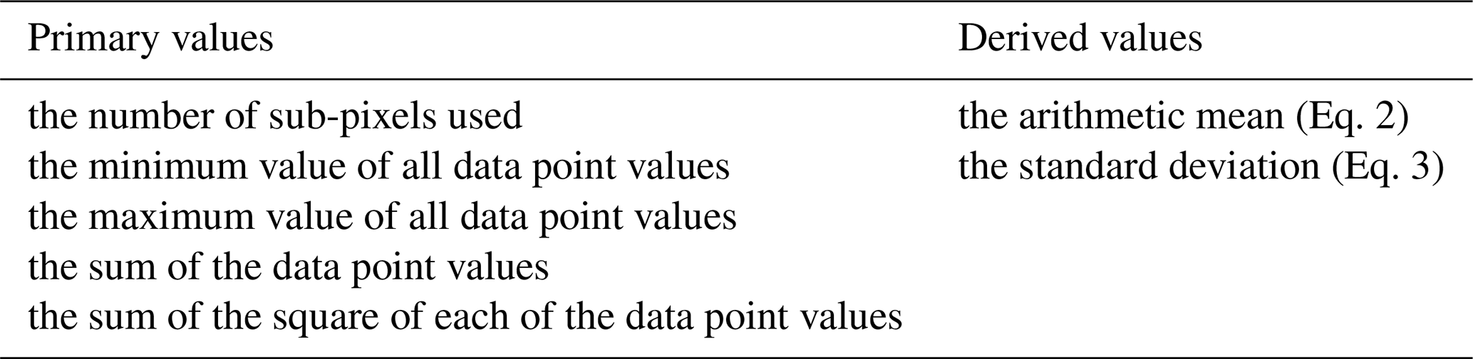
Table 2 lists the primary and derived values that are stored in the gridded ozone profile product.

Table 2 Primary and derived values stored in the gridded GOME-2 ozone profile product.

3.3 Gridded averaging kernel

As explained earlier in Sect. 2.3, the AK of the ozone profile describes the linear effect (weights) of ozone in all atmospheric layers on a particular (nominal) retrieved layer. In the level-2 ozone data, each individual retrieved profile has 40 layers and the associated AK matrix has 40×40 elements. While it is technically possible to store gridded/averaged AKs for all 0.25°×0.25° grid cells, this would make a regular level-3 gridded data product 40 times larger and unwieldy to use. As an alternative we have chosen to grid/average all AKs in 18 bands of 10° latitude.

An example of such a gridded/averaged AK is shown in Fig. 1, where for March 2019 the GOME-2B AK matrix for the latitude band at 45° N is shown on the left, and the smoothing weight curves for the nominal layers are shown in the middle. In the matrix plot, the x-axis (x_i) can be seen as the nominal retrieved layer index, and the y-axis then represents the index of the smoothing weights of the contributing layers to the particular nominal layer at index x_i. Also shown in Fig. 1 on the right is the ozone profile and a priori profile at 45° N/0° E for the same month, which gives a perspective in the shape of the profile and the position of the ozone maximum in the gridded data.

What stands out is that the bottom four layers have very little sensitivity (the matrix values are green across the vertical). In other words: the GOME-2 retrieved ozone profile is not very sensitive in the troposphere where (on average) relatively little ozone is present. For the next few layers, there is a positive sensitivity close to the nominal (indexed) layer, and a negative or positive weight higher up. Above layer 15 (31 hPa), the positive values start a little above the diagonal, which means that the profile is more sensitive to ozone above the nominal layer. For the top eight layers there is also little sensitivity, which corresponds with the upper stratosphere with diminishing ozone as one goes up.

In order to assess the the impact of these positive and negative effects indicated in the AK, we should also take into account the ozone content at those layers location. Even though the weights of the AK curves are fanning out at the top layers, their impact on the retrieved value is relatively small because there is very little ozone above layer 30 (1 hPa).

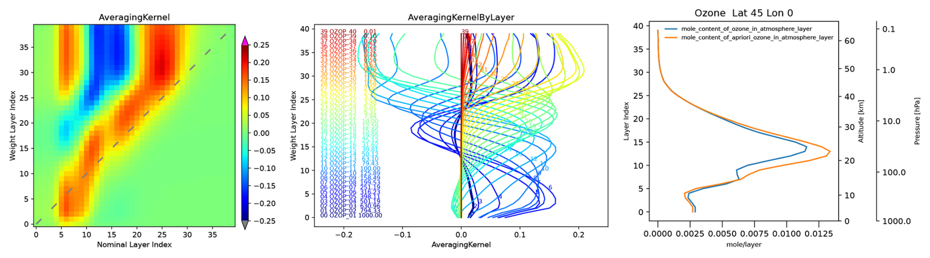
Figure 1 Example of the gridded averaging kernel, for GOME-2B at 45° N, (i.e. the 40–50° N band) on March 2019. Left: the whole averaging kernel; Middle: the averaging kernel curves of the individual layers; Right: the ozone profile and a priori at 45° N/0° E in mole for the layer. In the left panel there is a dashed line indicating the diagonal.

As mentioned above, we longitudinally average the AKs so they are representative for bands of 10° latitude in order to save space in the output product. While this is unconventional, a study done by Johnson et al. (2018) shows that using a representative AK results in relatively small differences in a wide range of ozone profile cases (generally <5 %–10 % across the whole profile). To explore this a little further, we present as an example the variability of the averaging kernels in the 40–50° N latitude band in Fig. 2. This figure shows the mean of the colocated averaging kernels (top) and the 10th, 50th and 90th percentiles (bottom row) of a full year of level-2 GOME-2A ozone profile retrievals in the 40–50° N latitude band. The percentile plots provide an indication of the spread of the AK values in the level-2 data used as a source for the level-3. While the change in the AK value along the percentiles is most prominent in the upper stratosphere (above layer 25 (3 hPa)), this is also the region with diminishing ozone and therefore has a smaller effect on the retrieved ozone. At the same time, the main structure along the diagonal remains intact across the whole range of percentiles in the altitude region where most of the ozone is present. The mean and median (i.e. the 50th percentile) of the averaging kernels are very similar, so in the level-3 gridded product we provide the mean because of ease of calculation. In the Appendix A, the 10th, 50th and 90th percentile are shown for all 18 latitude bands for 2009 as a reference.

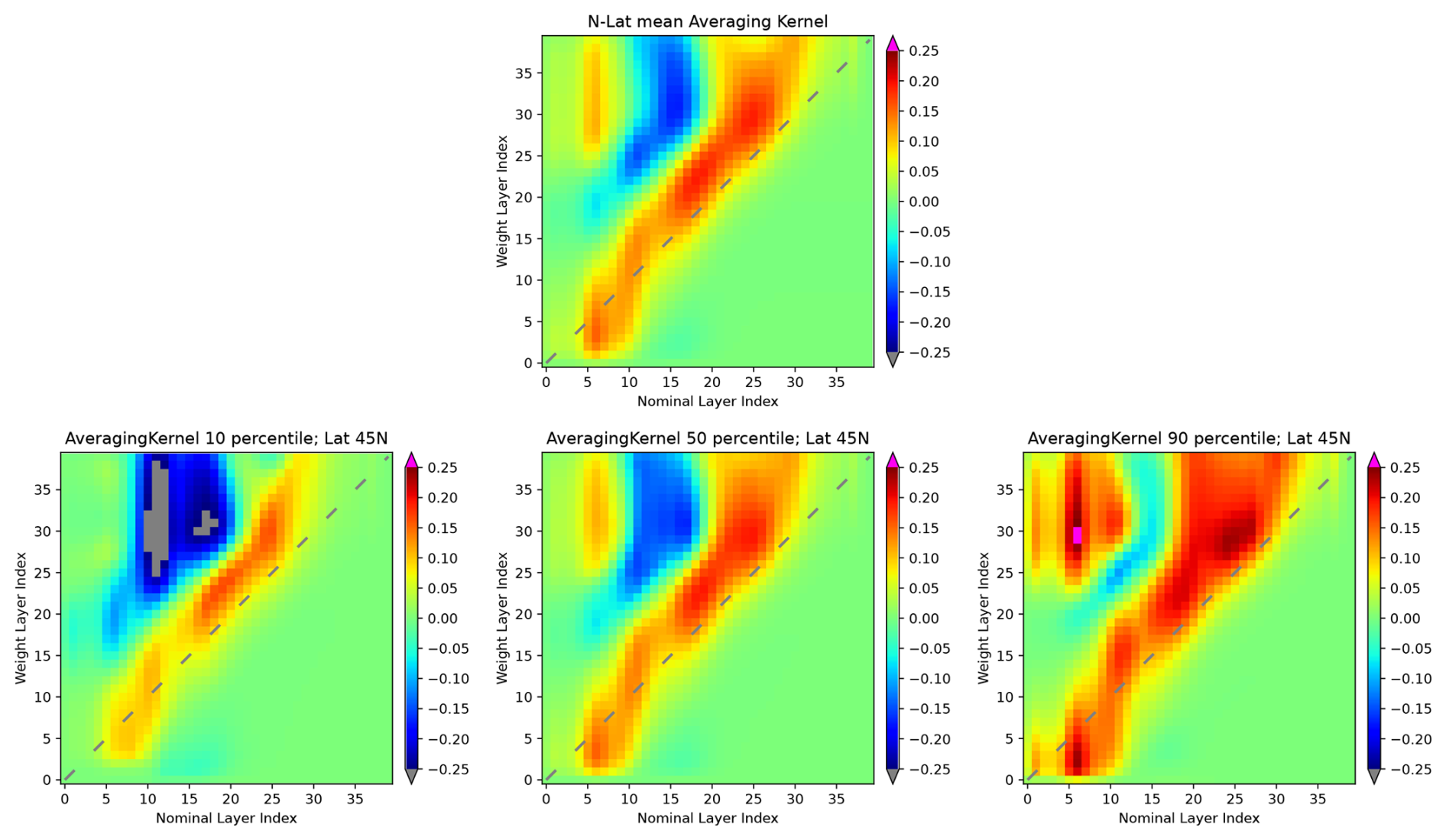
Figure 2 Averaged averaging kernels of GOME-2A ozone profile retrievals in the 40–50° N latitude band in 2009: the mean (top), and the 10th, 50th and 90th percentile (bottom row). The gray dashed lines represent the diagonal.

3.4 Time series of parameters

Figure 3 shows a time series of the global arithmetic mean of some of the parameters in the level-3 data set, which give a general impression of its behaviour over the mission period. It shows the atmosphere mole content of ozone (i.e.: the full atmosphere), the atmosphere mole content of the lower troposphere (surface to 500 hPa), the number of spectral detector pixels used in the (level-2) retrieval and the degrees of freedom of the resulting profile (the DFS is the trace of the averaging kernel). Due to specific validity of the spectral ranges of each of the GOME-2 instruments, the number of spectral pixels (NMeasurements) is also different. The degradation of the GOME-2 instrument contributes to a reduction of valid spectral information going into the level-2 retrieval over time. In the case of GOME-2A, the degradation (and quality control of the spectrum) causes an increasingly steep drop-off of the number of valid spectral information of GOME-2A after 2018. The effect of this can be seen in an increasing deviation of the total ozone column compared to the other instruments, and especially in the troposphere. The degradation in general also has an effect on the degrees of freedom of the retrieval. The DFS of GOME-2A has a discontinuity around September 2009, when an instrument de-contamination attempt caused a permanent degradation of the transmission and sensing of light through the instrument and detector.

Even though the retrieved level-2 and gridded level-3 data is available to users, we recommend to not use the ozone data from GOME-2A after 2018 and restrict our validation of this instrument therefore up to the end of that year.

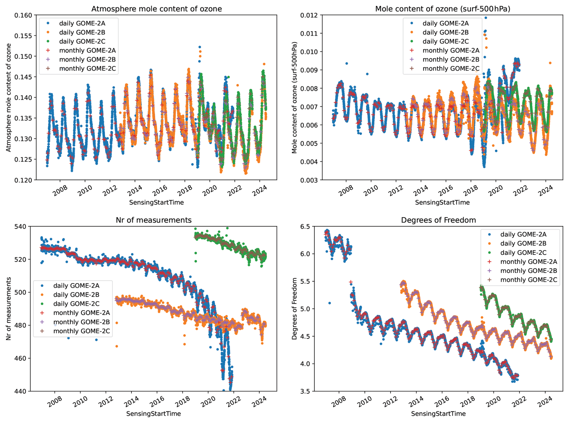
Figure 3 Time series of the global arithmetic mean of some parameters from GOME-2A/B/C jointly for the full available data length in the data record. Both the daily global mean is shown as well as the monthly mean. Top left: mole content of ozone (full vertical column), top right: mole content of ozone from the surface to 500 hPa, bottom left: number of spectral detector pixels used in the retrieval, bottom right: number of degrees of freedom in the retrieval.

4 Validation Data and Methods

The quality assessment of the AC SAF GOME-2A/B/C gridded ozone profile products was carried out using independent ground-based observations. For the lower stratosphere, UTLS and troposphere, comparisons were made with ozonesonde measurements. Ozonesondes are balloon-borne instruments capable of measuring vertical ozone profiles from the surface up to approximately 30 km, with a much higher vertical resolution (∼180 m) than satellite sensors (WMO, 2018). In addition, ozonesondes generally provide better precision and accuracy in the lower stratosphere and troposphere. They can also be launched under nearly all meteorological conditions and at any time of day. The precision of ozonesonde measurements varies with altitude and depends on the type of instrument (Stauffer et al., 2022). For this validation study, only the ozonesonde station of Hohenpeissenberg still uses Brewer-Mast ozonesondes. For the Japanese stations KC sondes were operational until December 2009. The other stations used (Fig. 4) in this validation study are all using ECC ozonesondes. Intercomparison campaigns and quality assurance studies have demonstrated systematic differences in precision between electrochemical concentration cell (ECC) and Brewer–Mast (BM) ozonesondes across the troposphere and stratosphere. In the troposphere (surface to ∼ 10 km; ∼ 1000–300 hPa), ECC sondes exhibit high precision, typically within ±3 %–4 % (Stubi et al., 2008; Smit et al., 2007, 2011). In the lower to mid-stratosphere (10–30 km; ∼ 300–10 hPa), ECC sondes maintain excellent precision of approximately ± 3 % across different manufacturers and cathode sensing solutions, while BM sondes show moderate precision of ± 3 %–5 % (Stubi et al., 2008; Smit et al., 2011). In the upper stratosphere (30–35 km; ∼ 10–1 hPa), ECC sondes continue to perform well, with uncertainties slightly increasing to ∼ 3 %–4 %, with best performance reported around 40 hPa near the ozone maximum (Smit et al., 2007, 2011). Recent intercomparison work (Smit et al., 2024) indicates that for ECC ozonesondes the relative uncertainty remains in the order of 5 %–10 % throughout much of the profile, but rises at pressures below ∼ 13 hPa (∼ 30–32 km altitude). For the upper stratosphere (15–60 km), measurements from lidar, FTIR and MWR were used. These instruments extend vertical coverage beyond the range of ozonesondes and provide valuable overlap between 15 and 30 km. However, global coverage remains limited: only a few long-term lidar (approx. <5) and MWR (approx. <4) stations provide regular observations, often with significant delays in data availability. No long-term upper stratospheric observations are available from the southern polar regions.

Lidar systems, typically operating with the Differential Absorption Lidar (DIAL) technique (Godin et al., 1998), provide accurate ozone profiles in clear sky, nighttime conditions of up to about 50 km (Leblanc and McDermid, 2000; Steinbrecht et al., 2006). Usually, 5 to 8 profiles are acquired per month, each requiring several hours of integration depending on the system and the atmospheric conditions. The natural output format of lidar profiles is ozone number density versus geometric altitude.

MWRs retrieve ozone profiles by measuring the pressure-broadened shape of a thermal emission line (Lobsiger et al., 1984; Parrish et al., 1988). Using an optimal estimation technique (Rodgers et al., 1990), these instruments deliver ozone number density profiles typically between 20 and 60 km altitude. In contrast to lidar, MWRs operate during the day and are less affected by weather conditions. On average, 20 profiles are acquired per month, with integration times between 30 min and 5 h, depending on the instrument (Boyd et al., 2007; Hocke et al., 2007).

Table 3 Typical precision and vertical resolution of lidar, MWR, and FTIR ozone profile measurements as used for satellite validation (Steinbrecht et al., 2006; Vigouroux et al., 2015).

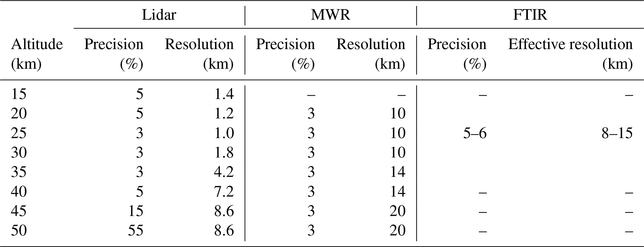
An FTIR spectrometer measures ozone profiles between 3 and 42 km by analyzing the interaction of infrared radiation with the atmosphere. The instrument records high-resolution infrared spectra. Ozone absorbs certain wavelengths of infrared light due to its molecular structure. The FTIR spectrometer detects this absorption and converts the information into an ozone profile using the Fourier transform method. This conversion allows ozone concentrations to be represented as a function of altitude. Note, FTIR ozone profile retrievals provide independent information typically limited to 2 to 4 degrees of freedom, corresponding to an effective vertical resolution of about 8–15 km in the stratosphere. The total error range is from 1.5 % to 2.5 % between 250 and 300 DU (Vigouroux et al., 2015; Garcia et al., 2022) without a simultaneous temperature fit, but around 1.5 % when a temperature retrieval is included in the data retrieval.

4.1 Ground-based Dataset Description

Ground-based ozonesonde observations used in this study are available from the World Ozone and Ultraviolet Data Center (WOUDC, http://www.woudc.org, last access: 20 March 2026) and the NILU Atmospheric Database for Interactive Retrieval (NADIR) hosted by the Norwegian Institute for Air Research (NILU, https://ebas.nilu.no, last access: 25 March 2026). Ground-based lidar, FTIR and MWR ozone profiles were obtained from the Network for the Detection of Atmospheric Composition Change (NDACC, https://ndacc.larc.nasa.gov/, last access: 23 March 2026). All NDACC lidar, FTIR, and MWR instruments undergo a standardized evaluation process and extensive quality control (Keckhut et al., 2004).

Figure 4 provides an overview of the stations used for this validation. Ozonesonde stations are indicated by crosses, lidar stations by triangles, FTIR stations by circles, and MWR stations by squares. The latitudinal classification is as follows: northern polar stations (green, 67–90° N), northern mid-latitude stations (black, 30–67° N), tropical stations (red, 30° N–30° S), southern mid-latitude stations (gray, 30–70° S) and southern polar stations (blue, 70–90° S). For each station, we computed a monthly mean ground-based ozone profile, and compared it to the monthly mean level-3 ozone data obtained with a horizontal distance smaller that 100 km around the location of the ground-based stations.

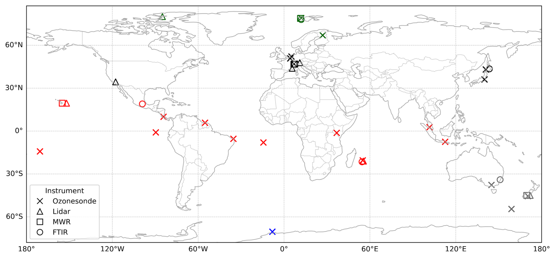
Figure 4 Overview of the stations used for tropospheric and stratospheric quality assessment. Ozonesonde stations are indicated by crosses, lidar stations by triangles, FTIR by circles, and MWR stations by squares. The latitudinal classification is: northern polar stations (green, 67–90° N), northern mid-latitude stations (black, 30–67° N), tropical stations (red, 30° N–30° S), southern mid-latitude stations (grey, 30–70° S), and southern polar stations (blue, 70–90° S).

4.2 Pre-processing of ground-based ozone profile Data and Application of Satellite Averaging Kernels

The ground-based ozone lidar, FTIR, and MWR profiles were pre-processed and harmonized with the satellite retrieval grid in order to enable a consistent comparison. The lidar, FTIR, and MWR data files contain monthly mean ozone number densities (cm⁻³) between approximately 15 and 50 km. The lidar, FTIR, and MWR profiles were converted into partial ozone columns expressed in Dobson Units (DU) per layer according to:

$$\begin{array}{}\text{(6)}& {\mathrm{DU}}_{\mathrm{layer}}={\displaystyle \frac{n\left(z\right)\mathrm{\Delta }{z}_{\mathrm{cm}}}{\mathrm{2.687}\times {\mathrm{10}}^{\mathrm{16}}}},\end{array}$$

where n(z) is the ozone number density (in cm⁻³) and Δz_cm is the layer thickness in centimeters.

For each month, the corresponding satellite data (retrieved ozone, a priori ozone, averaging kernel, and standard deviation) were extracted from the level-3 NetCDF ozone profile data record files. The satellite quantities, given as ozone column amounts in mol m⁻², were converted into Dobson Units by using $\mathrm{1}\mathrm{DU}=\mathrm{4.462}\times {\mathrm{10}}^{-\mathrm{4}}\mathrm{mol}{\mathrm{m}}^{-\mathrm{2}}$. Ozonesonde data, already available in DU, were integrated over the GOME-2 pressure layers. The vertical coordinates of the satellite layers, originally defined in pressure, were converted to geometric altitude using the U.S. Standard Atmosphere (1976).

The averaging kernels (AKs) provided with the satellite product were applied to the ground-based ozone profiles from lidar, MRW, and ozonesonde following the standard smoothing approach described by Eq. (1). Specifically, the smoothed ground-based profile ${\widehat{\mathit{x}}}_{\mathrm{gb}}$ was calculated following Rodgers (2000) as ${\widehat{\mathit{x}}}_{\mathrm{gb}}={\mathit{x}}_{\mathrm{a}}+\mathbf{A}({\mathit{x}}_{\mathrm{gb}}-{\mathit{x}}_{\mathrm{a}})$, where x_gb denotes the original ground-based ozone profile, x_a the satellite a priori profile, and A the satellite averaging kernel. This operation ensures that the ground-based profiles are smoothed to the vertical sensitivity and smoothing characteristics of the satellite retrieval. All ozone profiles (satellite retrieved, a priori, ground-based, and smoothed ground-based) were subsequently interpolated and re-binned onto a uniform 1 km vertical grid up to 60 km altitude. The re-binning of partial columns from the irregular satellite layers to the uniform grid conserved the total amount of ozone in DU by weighting each layer according to the geometric overlap between the native and target bins. The described processing ensures that the ground-based profiles are expressed on the same vertical grid and smoothing characteristics as the satellite retrievals, thus allowing a direct and consistent validation of the satellite ozone profiles. FTIR ozone profiles are themselves retrieval products characterized by their own averaging kernels and a priori profiles. To ensure a consistent comparison with the level-3 satellite retrievals, a bidirectional averaging-kernel approach is applied following Rodgers and Connow (2003). In this framework, the satellite averaging kernels are applied in the Dobson Unit (DU) domain to the FTIR profiles while explicitly accounting for the FTIR a priori state. This procedure minimizes inconsistencies that arise from differences in vertical resolution and retrieval characteristics between the two data sets. Such treatment is consistent with established methodology for intercomparison of retrieval products with differing vertical sensitivities (Calisesi et al., 2005). A comparable strategy has been applied in previous satellite validation studies involving FTIR data, for example, in the validation of IASI ozone products using GOME-2 and ground-based observations (Boynard et al., 2018), where the role of averaging kernels and a priori information in profile comparisons is explicitly addressed. For high-vertical-resolution reference measurements (lidar and ozonesondes), only the satellite averaging kernels are applied, as these measurements can be considered close approximations of the true atmospheric state.

For the validation the satellite data as well as the ground-based data were integrated over several altitude bands (e.g. 0–8, 8–14, 14–30, 30–40, and 40–50 km for mid-latitude levels). These band-integrated ozone columns were used to obtain time series for the ground-based, satellite, and smoothed ground-based datasets.

5 Validation of the GOME-2 Metop-A/B/C level-3 Ozone Profile Dataset

This section describes the validation of the reprocessed GOME-2A/B/C level-3 (gridded) ozone profile products. The validation periods are as follows: January 2007 to December 2018 for GOME-2A, December 2012 to December 2024 for GOME-2B, and January 2019 to December 2024 for GOME-2C.

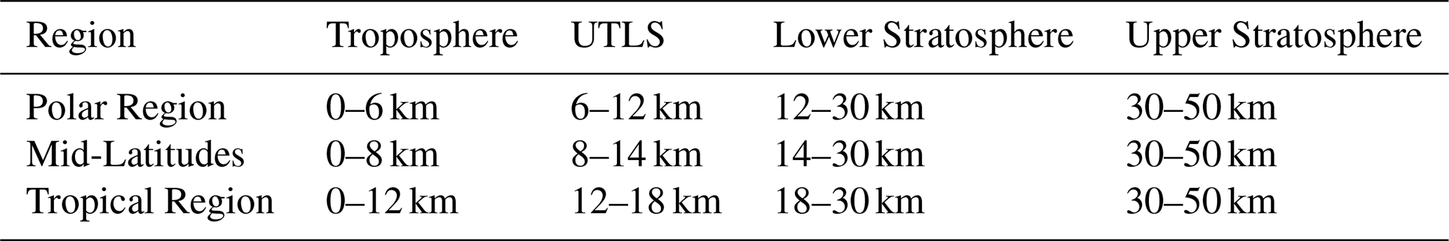
The validation is structured around the troposphere, UTLS, lower stratosphere (up to 30 km altitude), and the upper stratosphere in different latitude bands (see Table 4).

Table 4 Definition of the vertical ranges for the latitude belts.

For the troposphere, UTLS and lower stratosphere, comparisons are made against ozonesonde measurements. For the upper stratosphere, lidar, FTIR, and microwave radiometer (MWR) data are used as reference. Relative differences are calculated using:

$$\begin{array}{}\text{(7)}& \text{RD}={\displaystyle \frac{{\mathrm{O}}_{\mathrm{3},\mathrm{L}\mathrm{3}}-{\mathrm{O}}_{\mathrm{3},\mathrm{AK}}}{{\mathrm{O}}_{\mathrm{3},\mathrm{AK}}}}\times \mathrm{100}\end{array}$$

where O_3,L3 indicates the ozone values in the gridded product, and O_3,AK indicates the ground-based reference ozone profile (either lidar, MWR, FTIR or balloon based) that is smoothed with the averaging kernel.

Table 5 GOME-2A/B/C gridded validation statistics (Absolute Difference [AD], Relative Difference [RD], and standard deviation [SD]) for the troposphere, UTLS-zone, lower and upper stratosphere across latitude regions: Units: AD in DU, RD and SD in %.

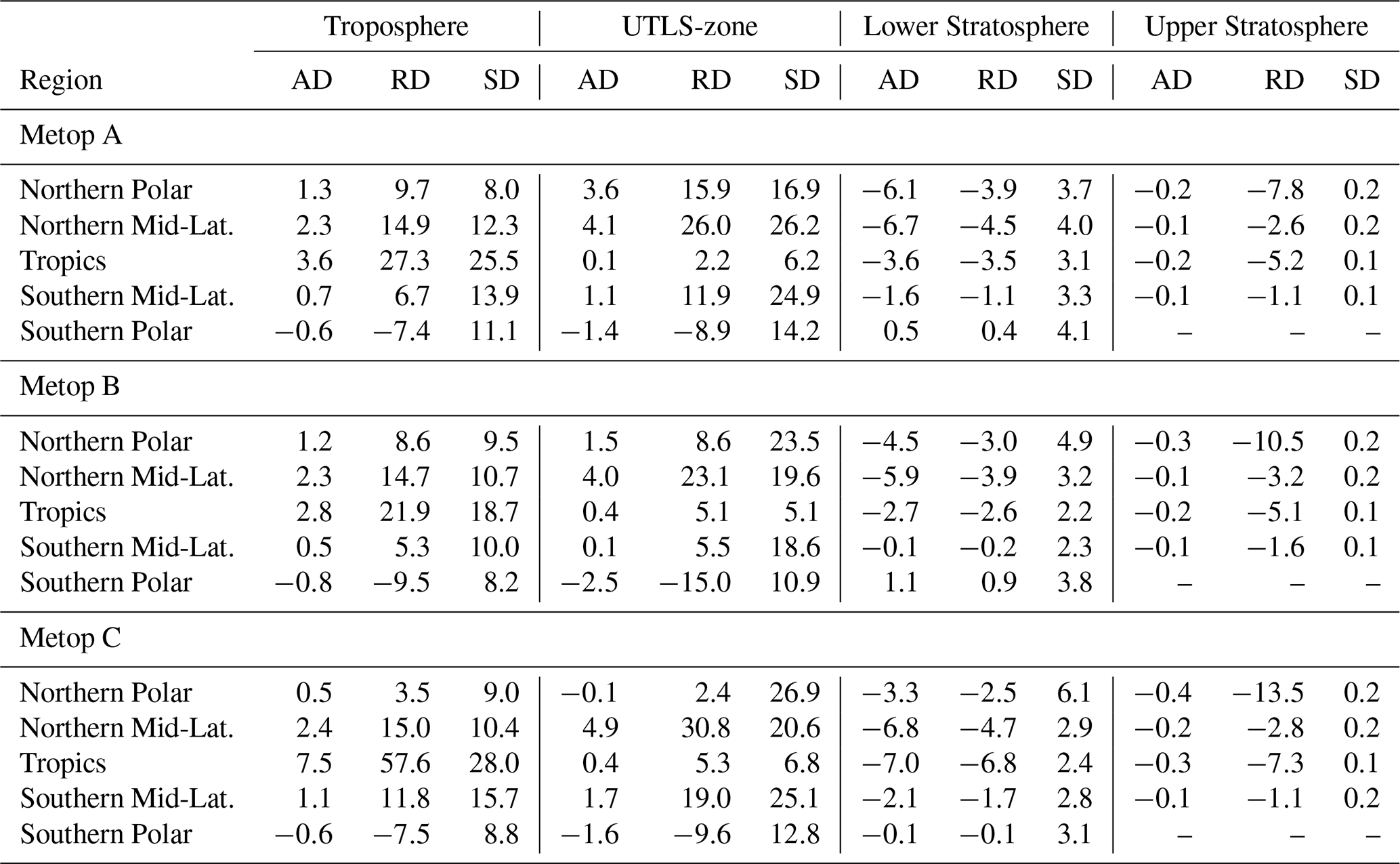
Table 5 summarizes the validation statistics for the different latitude belts, based on all available ground-based reference stations shown in Fig. 4. The statistics include contributions from lidar, microwave radiometer (MWR), FTIR, and ozonesonde observations, depending on data availability in the respective altitude ranges. For the upper stratospheric validation in the tropics, the analysis was limited to the period up to the end of 2022 due to the reduced availability of ground-based observations after 2022. The relative difference is generally below 15 % in the troposphere, except in the tropical troposphere, and both the lower and upper stratosphere for all latitude bands. For the southern polar stations, there was no information available for the upper stratospheric part. A station-to-station consistency analysis was performed using the mid-latitude stations as a representative example to assess the robustness of the validation results across independent reference data sets.

In the 30–40 km altitude range, the mean relative difference between the satellite product and the smoothed lidar observations at mid-latitude sites is approximately −3.5 %, with a station-to-station spread of about −3 % to −5 %. Comparisons with smoothed MWR observations yield a slightly smaller mean bias of about −2.8 %, with a comparable spread (−1.2 % to −4 %).

In the 40–50 km layer, the satellite-smoothed lidar differences increase to around −4 %, while the satellite-smoothed MWR differences remain closer to −2 %. Despite these differences in magnitude, the results from lidar and MWR observations are consistent in sign and order of magnitude, and all mean biases remain within approximately ±5 % for the mid-latitude stations.

Comparable bias magnitudes are found at the tropical sites (Fig. 4) for the lidar, FTIR, and MWR station. However, the Réunion lidar data above 40 km exhibit increased variability and reduced consistency compared to the other stations. As a result, these data are treated with caution and are not used as primary reference in the uppermost altitude range.

A comparison with the original (unsmoothed) ground-based data reveals substantially larger station-to-station variability and, in some cases, even a change in the sign of the bias. Applying the averaging-kernel-based smoothing markedly reduces these discrepancies, highlighting the importance of accounting for differences in vertical resolution in satellite-ground-based comparisons.

5.1 Validation results for the troposphere, UTLS and lower stratosphere

To assess the consistency of the GOME-2A/B/C level-3 ozone profile product in the troposphere, UTLS-zone and lower stratosphere, we compare the vertically integrated ozone partial profiles with the corresponding pressure levels derived from ozonesonde data, following Table 4. The averaging kernels are applied to high-resolution ozone profiles and those values are used in the evaluation. Table 5 summarizes the validation statistics as function of latitude and vertical regimes specified the three instruments respectively. In addition, Fig. 5 supplements the validation results from the mid-latitude stations in terms of time-series approach for the different latitude belts.

In the troposphere, all three GOME-2 instruments show predominantly positive biases in the Northern Hemisphere, with relative differences reaching 14 % to 15 % in the northern mid-latitudes for all sensors and up to 57.6 % in the tropics for Metop-C. Absolute differences in the northern mid-latitudes are consistently around 2 to 2.4 DU. Tropical biases are moderate for Metop-A and Metop-B (22 %–27 %) but substantially larger for Metop-C as earlier mentioned. In the southern mid-latitudes, positive biases are smaller (5 % to 12 %), while systematic negative biases are observed in the southern polar region (−7 % to −10 %). Overall, the tropospheric results indicate consistent Northern Hemisphere overestimation and enhanced variability compared to the UTLS, with notable inter-sensor differences in the tropics. For the UTLS region, all three GOME-2 instruments show consistent hemispheric differences. Positive biases are observed in the Northern Hemisphere, particularly in the northern mid-latitudes, where relative differences reach +26.0 % (Metop-A), +23.1 % (Metop-B), and +30.8 % (Metop-C), corresponding to absolute differences of 4 to 5 DU. For northern polar stations, the biases are smaller but remain positive for Metop-A and Metop-B, while Metop-C shows near-neutral absolute bias with elevated variability. In the tropics, all sensors exhibit small positive differences (2 % to 5 %) and low variability, indicating stable performance. In contrast, systematic negative biases are found in the southern polar region (−9 % to −15 %). For the lower stratosphere, the intercomparison with ozonesondes shows that all three sensors produce comparable results, with relative differences within 10 %. A seasonal dependence is observed in the dataset, consistent with the Level 2 product. Delcloo et al. (2024) also reported this seasonal dependence in both the lower stratosphere and the troposphere. In the lower stratosphere, all three instruments exhibit systematic negative biases in the Northern Hemisphere and tropics, with relative differences typically between −2.5 % and −6.8 % and absolute differences of −3 to −7 DU. The strongest negative biases are observed in the northern mid-latitudes for all sensors. In contrast, the southern polar region shows small positive or near-neutral differences (0 % to 1 %), while southern mid-latitude biases remain weakly negative. Variability is comparatively low across all latitude bands and markedly smaller than in the troposphere and UTLS. Overall, the lower stratospheric results demonstrate consistent underestimation in most regions but relatively stable performance with limited dispersion. For the first two years of the GOME-2A mission, there was a particular instrumental integration time setting for the spectral bands 1a and 1b in the far- and near-UV regions, that made it difficult to distinguish the troposphere from the stratosphere on small ground pixels. This was changed by the end of 2008 (also listed in Table 1). This instrument setting has affected the ozone profile across the full atmosphere for the first two years, but this effect should not cause the sustained bias for the first four years of the mission, as seen in Fig. 5. Our hypothesis is that the degradation correction, which spans multiple years in order to get the seasonal effect right, has a lingering effect.

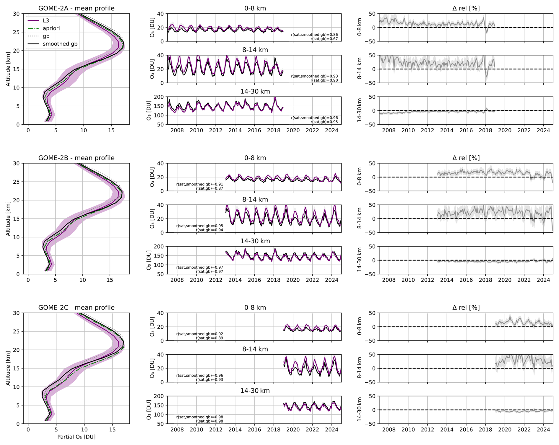
Figure 5 Comparison of ozone partial columns derived from satellite and ground-based observations for GOME-2A/B/C. For each sensor (from top to bottom), the three panels show: (left) the mean vertical profile of ozone partial columns in Dobson Units (DU) averaged over the entire observation period, including the level-3 satellite retrieval (purple), the ozonesonde measurement (grey), the ozonesonde profile smoothed by the satellite averaging kernel and a priori profile (black), the level-3 a priori profile (green), and the ±1σ uncertainty of the satellite profile (shaded); (middle) the time series of monthly mean ozone partial columns in the 0–8 km altitude range (troposphere), 8–14 km altitude range (tropopause). and in the 14–30 km altitude range (lower stratosphere) for the same data sources; and (right) the relative difference between the level-3 and smoothed ozonesonde data in this altitude range. This comprehensive comparison illustrates the consistency between satellite and ground-based ozone observations, as well as systematic differences over time and altitude.

5.2 Validation results for the upper stratosphere

To assess the consistency of the GOME-2 monthly mean level-3 ozone profile product in the upper stratosphere, monthly averaged satellite partial columns were compared with ground-based observations. In this altitude range, ground-based observations from lidar, MWR, and FTIR provide complementary information with different vertical sensitivities (see Table 3). The analysis focuses on the 30–50 km altitude range, where nadir-viewing UV instruments provide good sensitivity to stratospheric ozone due to Rayleigh scattering. However, when comparing vertically resolved ozone profiles or partial columns in narrow altitude ranges, differences in vertical resolution and smoothing between satellite and ground-based observations need to be taken into account. Therefore, the application of the averaging kernel is required to ensure a consistent comparison between satellite and ground-based profile measurements. This is consistent with previous studies showing that averaging-kernel effects are less critical for total or broad stratospheric column ozone but become important for profile-based or layer-resolved comparisons (e.g., Liu et al., 2010; Keppens et al., 2024). The results of the comparison for mid-latitude and tropical stations are presented in Figs. 6 and 7, respectively. The mean smoothed ground-based profiles (left panel) closely follow the satellite retrievals, particularly between 40 and 50 km.

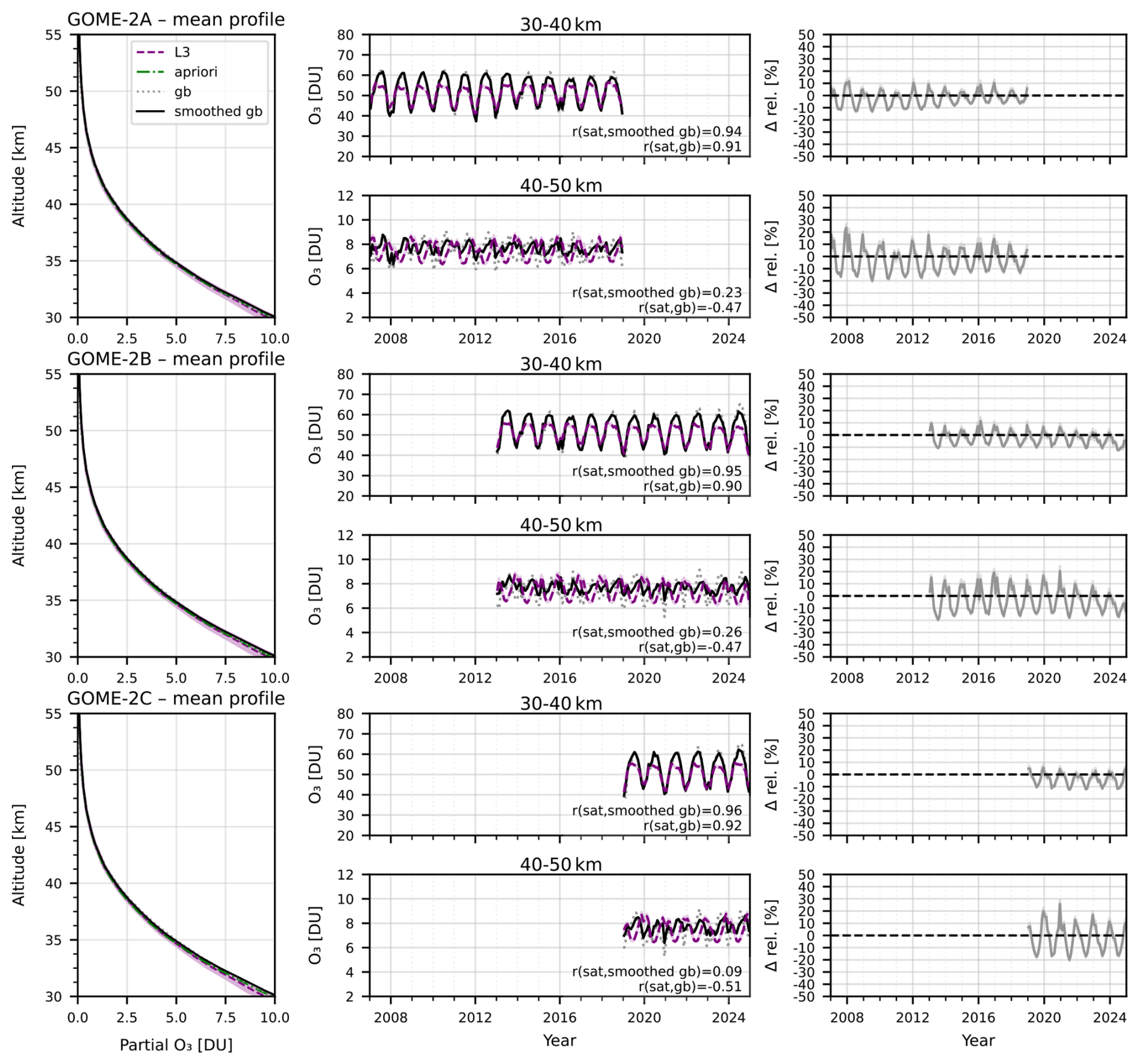
Figure 6 Comparison of satellite derived ozone partial columns and all mid-latitude ground-based observations as shown in Fig. 4. Top to bottom: GOME-2 A/B/C instrument. Left: the mean vertical profile of ozone partial columns in DU (purple), the ground-based measurement (grey), the smoothed ground-based profile (black), the level-3 a priori profile (green), and the ±1σ uncertainty of the satellite profile (shaded); Middle: the time series of monthly mean ozone partial columns for the 30 to 40 and 40 to 50 km altitude ranges for the same data sources with the Pearson correlation coefficient (r) between the level-3 and ground-based as well as smoothed ground-based time series; Right: the relative difference between the level-3 and smoothed data in this altitude range.

Figure 7 Same as Fig. 6 but for all tropical ground-based stations as shown in Fig. 4.

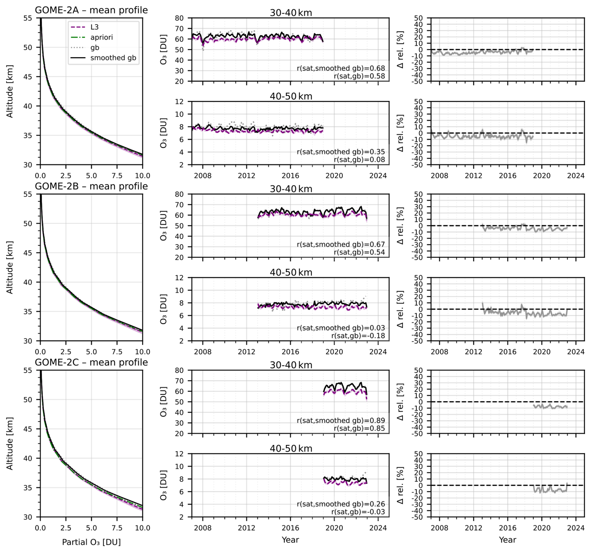
The time series of monthly mean ozone partial columns between 30–40 and 40–50 km (middle panels) show good agreement in both long-term variability and seasonal cycles, with maxima in summer and minima in winter. In the 40–50 km layer, the overall seasonal behavior is also reproduced, although a systematic phase shift between the satellite and ground-based time series is apparent. Although a bias in absolute values is apparent between the satellite and ground-based datasets, the satellite product reliably reproduces the temporal evolution of ozone in the upper stratosphere. The correlation coefficients for each altitude range are indicated in the middle panels. The higher correlation between the smoothed ground-based and level-3 time series, compared to that between the original ground-based and level-3 data, highlights the effectiveness of the apriori and averaging kernel-based smoothing in taking into account differences in vertical resolution. Here r denotes to the correlation coefficient calculated from the monthly mean time series. In the 40–50 km altitude range, the combination of narrow layer integration, occasional crossings of satellite and ground-based profiles, and the increased influence of the apriori profile can lead to reduced or even negative correlation coefficients, despite the overall consistency of the mean profiles. Such behavior is a known feature of nadir profile retrievals, where the vertical sensitivity and averaging kernels redistribute information across the profile and relative to the apriori, affecting the apparent temporal phasing and trend structure when compared to high-vertical-resolution references (Keppens et al., 2015; Rivoire et al., 2025).

The relative bias (left panels in Figs. 6 and 7) between the three satellite sensors and the smoothed ground-based data (right panels) remains within ± 10 % in the 30–40 km altitude range. In the 40–50 km region, the relative differences are larger, around 20 %, particularly during periods of ozone maxima and minima. Nevertheless, the mean relative difference, as reported in Table 5, is below 5 %. Overall, the ground-based validation confirms the robustness of the GOME-2 level-3 ozone profile product and its suitability for cross-validation with other satellite datasets and the construction of long-term ozone time series.

5.3 Inter sensor differences

Figure  8 illustrates the inter-sensor differences between the three GOME-2 instruments respectively in the upper stratosphere for the altitude ranges 30–40 km (gray line) and 40–50 km (black line). Figure 9 is showing this for the troposphere within the altitude range 0–8 km (gray line) and for the lower stratosphere within the altitude range 14–30 km, averaged across all mid-latitude stations. The comparison reveals a high degree of consistency among the sensors. The smallest discrepancies are observed in the 40–50 km layer, indicating robust long-term stability in this altitude range. It is also shown in Fig. 9 that for GOME-2A, the data after 2018 is not consistent anymore and should not be used after that date.

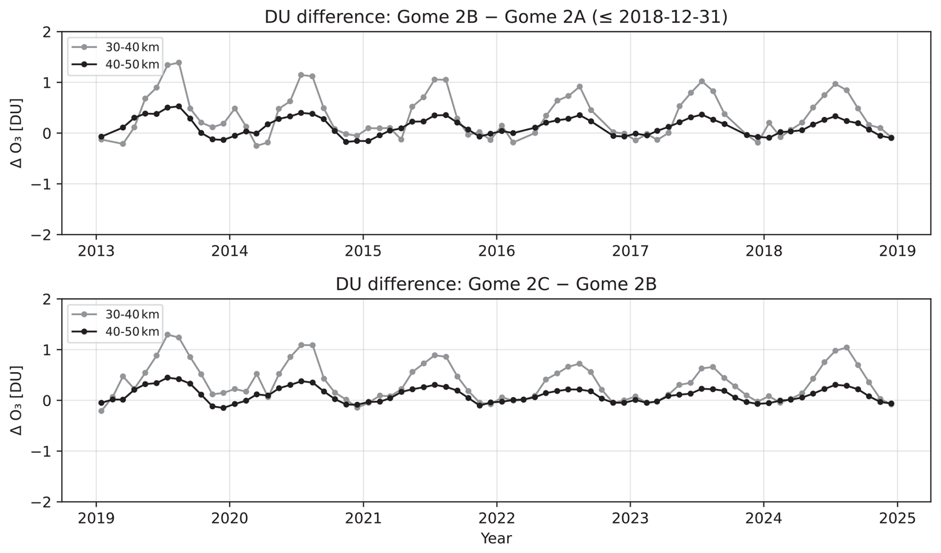
Figure 8 Time series of differences in partial ozone columns (DU) between the GOME-2 satellite pairs for two altitude ranges. Top: GOME-2B minus GOME-2A, limited to the period up to 31 December 2018 due to the reduced data quality of GOME-2A. Bottom: GOME-2C minus GOME-2B over the respective overlapping time period. Both panels show the altitude ranges 30–40 km (gray line) and 40–50 km (black line).

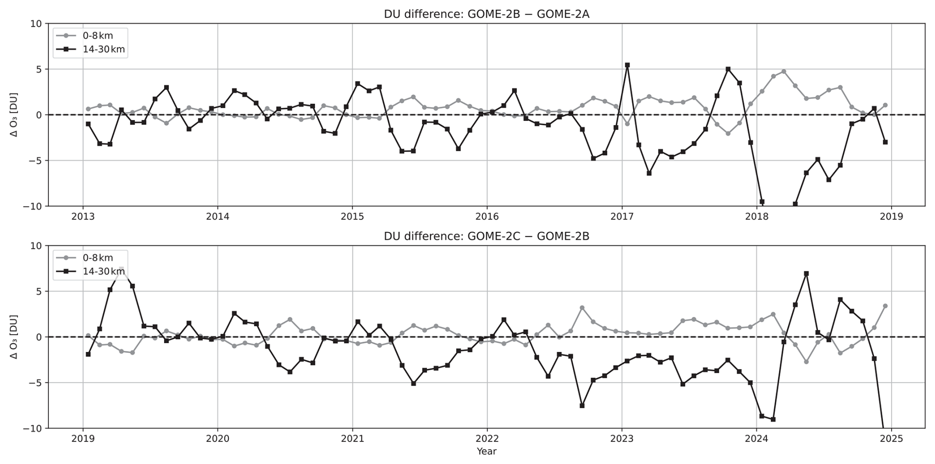
Figure 9 Time series of differences in partial ozone columns (DU) between the GOME-2 satellite pairs for two altitude ranges. Top: GOME-2B minus GOME-2A, limited to the period up to 31 December 2018 due to the reduced data quality of GOME-2A. Bottom: GOME-2C minus GOME-2B over the respective overlapping time period. Both panels show the altitude ranges 0–8 km (gray line) and 14–30 km (black line).

6 Conclusions

A comparison study of ozone retrieval statistics from the GOME-2 instruments onboard of Metop-A, -B, and -C shows a high level of consistency across latitude bands and atmospheric layers, confirming the maturity and stability of the retrieval algorithm. In the troposphere, all three sensors tend to slightly overestimate ozone, with absolute differences (AD) of roughly +1 to +3 DU in mid-latitudes and up to +7.5 DU in the tropics for Metop-C. Relative differences increase toward lower latitudes, reflecting higher retrieval uncertainty under variable cloud and humidity conditions. In the UTLS, GOME-2 instruments show positive biases in the Northern Hemisphere, largest in mid-latitudes, and negative biases in the southern polar region. Tropical biases are small (2 % to 5 %) with low variability, while mid- and high-latitude variability is higher (up to 27 %). In the lower stratosphere, all sensors show a small negative bias, typically between −3 and −7 DU (RD ≈−3 % to −7 %), corresponding to a modest underestimation of ozone concentrations. The lowest scatter is observed for Metop-B. In the upper stratosphere, biases are minimal across all sensors, with absolute difference values, close to zero (−0.1 to −0.4 DU) and extremely low variability (SD ≈0.1 to 0.2 DU). These results confirm excellent consistency in the upper-stratospheric ozone retrievals, where radiometric calibration and spectral fitting are least affected by tropospheric interference.

The observed inter-sensor consistency across Metop-A, -B, and -C supports the creation of a coherent, multi-decadal ozone climate data record. Minor biases in the troposphere and lower stratosphere are small relative to natural ozone variability and can be corrected through standard inter-calibration procedures. The minimal deviations in the upper stratosphere further reinforce the stability of GOME-2 instruments over time, making the Metop constellation a reliable backbone for long-term monitoring of ozone distribution, stratosphere-troposphere interactions, model evaluations and assessment of policy-driven ozone recovery. In conclusion, these results confirm the use of merged Metop GOME-2 datasets in constructing consistent, high-quality ozone time series, suitable for climate and atmospheric research.

Appendix A: Averaged Averaging Kernels by latitude band

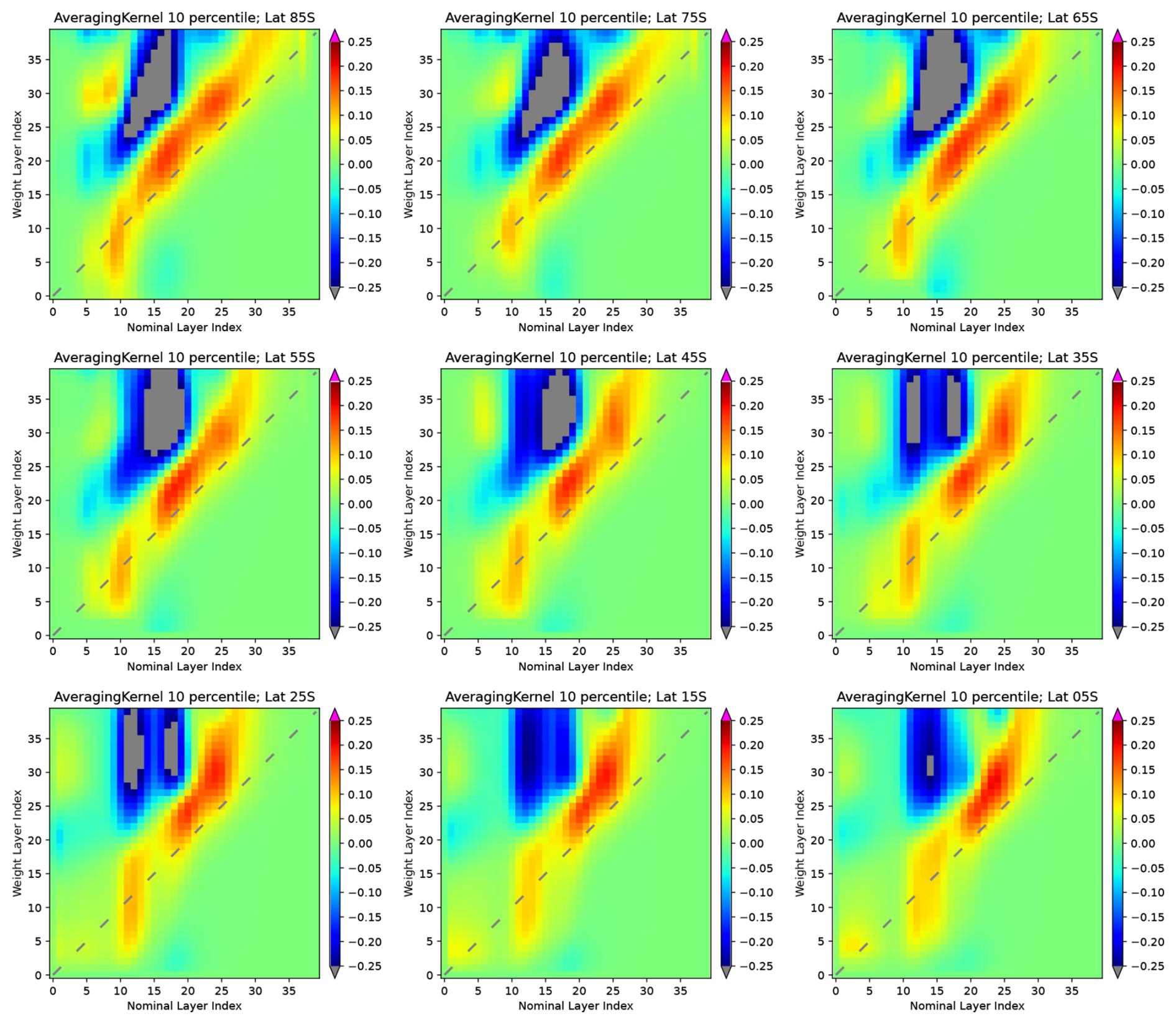
Figure A1 10th percentile of the averaged averaging kernels of GOME-2A by 10° latitude band in 2009 (Northern Hemisphere).

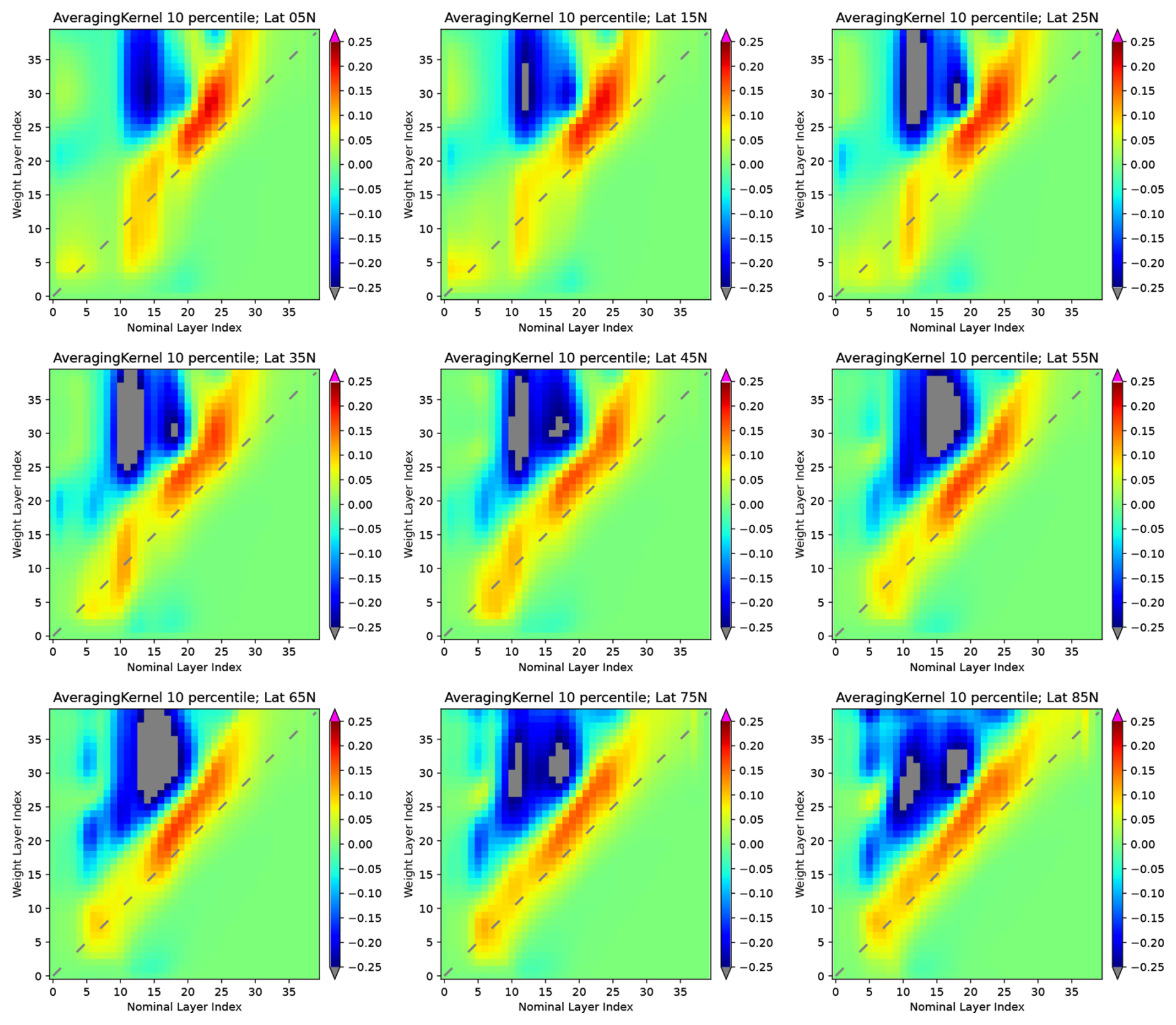
Figure A2 10th percentile of the averaged averaging kernels of GOME-2A by 10° latitude band in 2009 (Southern Hemisphere).

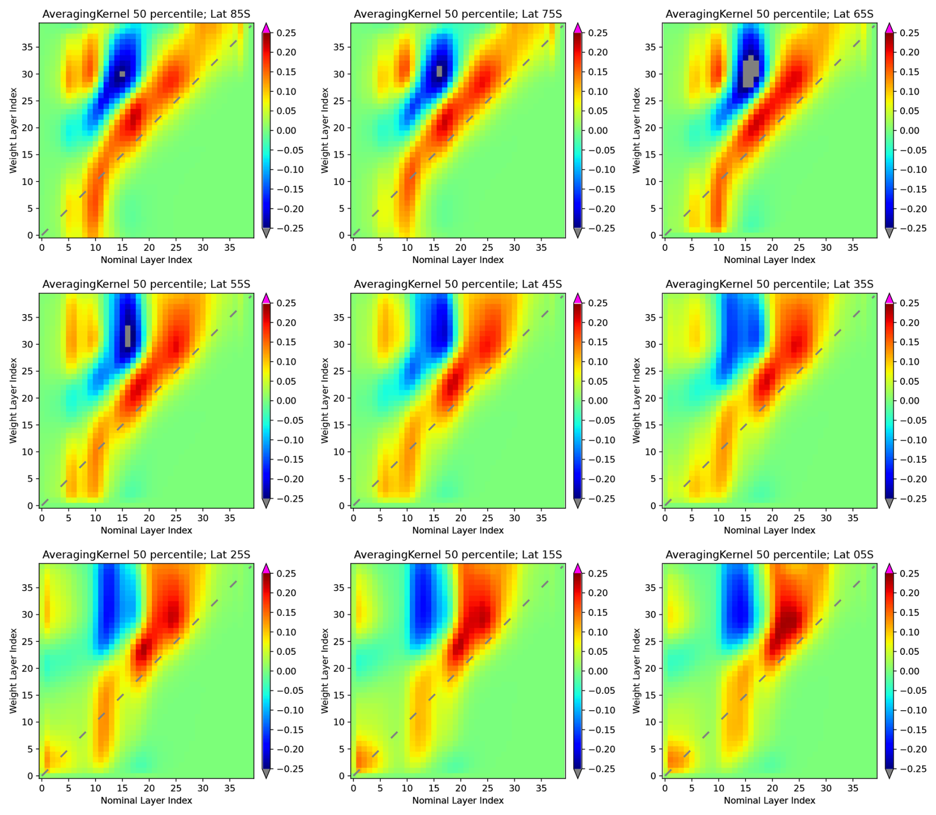
Figure A3 50th percentile of the averaged averaging kernels of GOME-2A by 10° latitude band in 2009 (Northern Hemisphere).

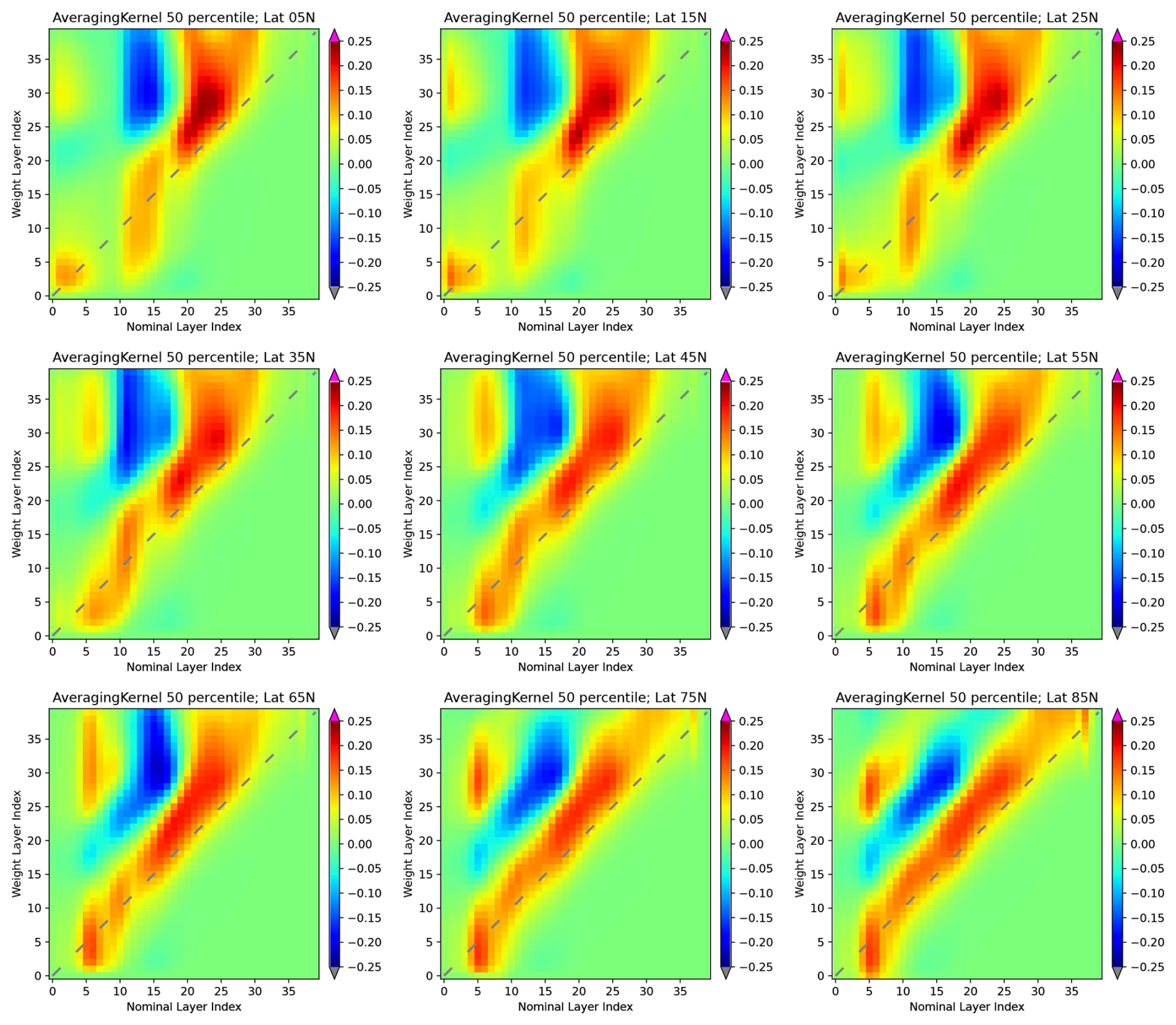
Figure A4 50th percentile of the averaged averaging kernels of GOME-2A by 10° latitude band in 2009 (Southern Hemisphere).

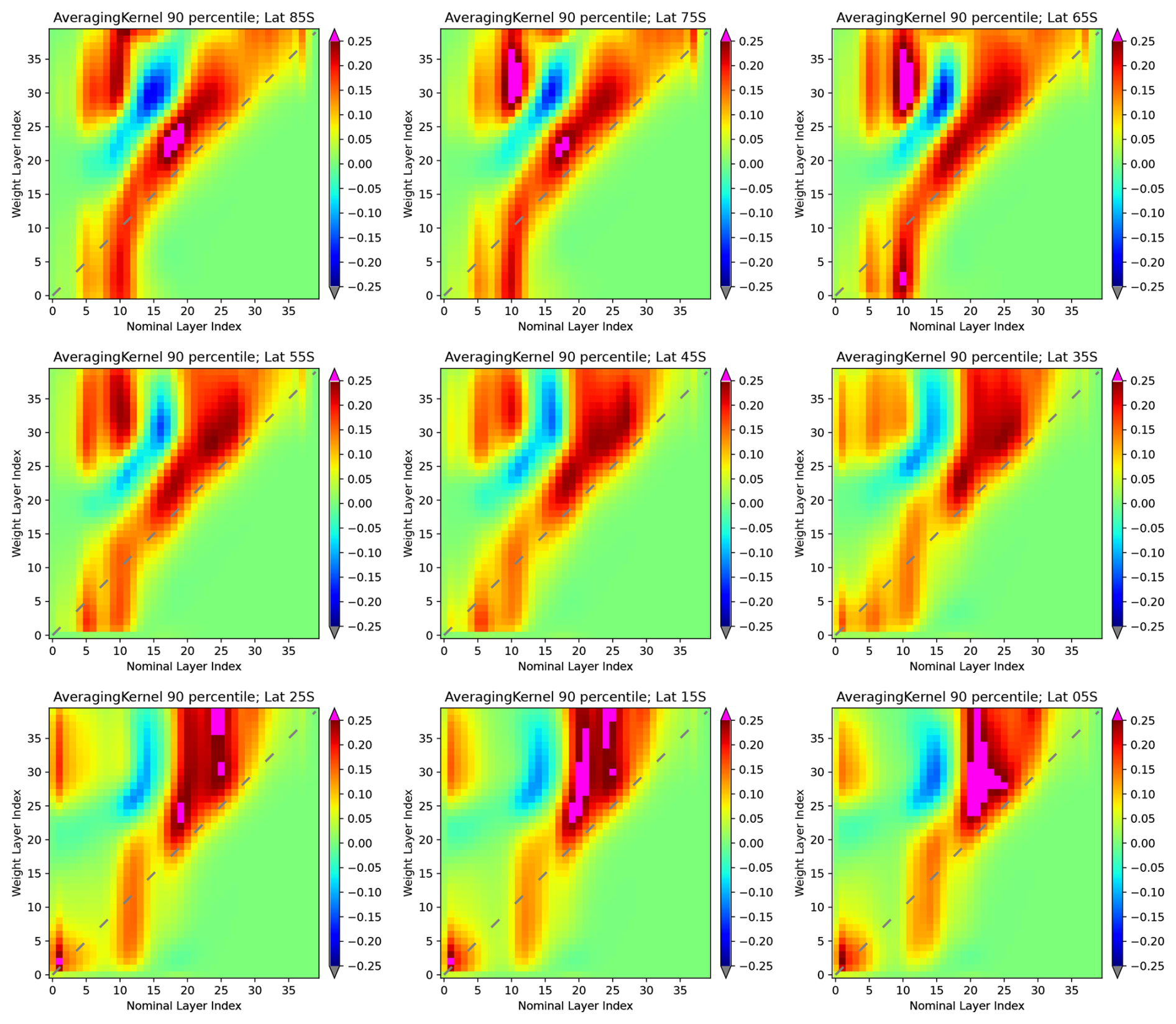
Figure A5 90th percentile of the averaged averaging kernels of GOME-2A by 10° latitude band in 2009 (Northern Hemisphere).

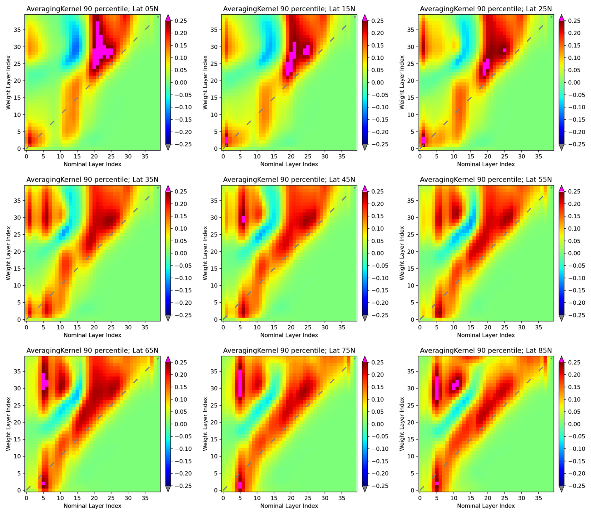
Figure A6 90th percentile of the averaged averaging kernels of GOME-2A by 10° latitude band in 2009 (Southern Hemisphere).