Model-based climatology of diurnal variability in stratospheric ozone as a data analysis tool

Observational studies of stratospheric ozone often involve data from multiple instruments that measure the ozone at different times of day. There has been an increased awareness of the potential impact of the diurnal cycle when interpreting measurements of stratospheric ozone at altitudes in the mid- to upper stratosphere. To address this issue, we present a climatological representation of diurnal variations in ozone with a 30 min temporal resolution as a function of latitude, pressure and month, based on output from the Goddard Earth Observing System (GEOS) general circulation model coupled to the NASA Global Modeling Initiative (GMI) chemistry package (known as the GEOS-GMI chemistry model). This climatology can be applied to a wide range of ozone data analyses, including data intercomparisons, data merging and the analysis of data from a single platform in a non-sun-synchronous orbit. We evaluate the diurnal climatology by comparing mean differences between ozone measurements made at different local solar times to the differences predicted by the diurnal model. The ozone diurnal cycle is a complicated function of latitude, pressure and season, with variations of less than 5 % in the tropics and subtropics, increasing to more than 15 % near the polar day terminator in the upper stratosphere. These results compare well with previous modeling simulations and are supported by similar size variations in satellite observations. We present several example applications of the climatology in currently relevant data studies. We also compare this diurnal climatology to the diurnal signal from a previous iteration of the free-running GEOS Chemistry Climate Model (GEOSCCM) and to the ensemble runs of GEOS-GMI to test the sensitivity of the model diurnal cycle to changes in model formulation and simulated time period.

1 Introduction

Stratospheric ozone has been an environmental concern since the suggestion 45 years ago that anthropogenic chemicals (collectively known as ozone depleting substances; ODSs) released into the atmosphere could destroy ozone (Stolarski and Cicerone, 1974; Molina and Rowland, 1974). Since that time, our understanding of ozone chemistry and dynamics has vastly evolved, and high quality satellite and ground-based observations of ozone have been key to that evolution. These observations were used to quantify ozone loss during the 1980s and early 1990s and are now being used to quantify the turn around and expected increase in ozone after the ban of many ODSs. However, the slow decline in these chemicals, resulting from their long atmospheric lifetimes and the staged reduction of their use through the Montreal Protocol and subsequent amendments, means that the ozone recovery rate will be much slower than the loss rate. Therefore, observations must be sufficiently stable to resolve these small changes in time. Furthermore, measurements from more than one source are required to provide adequate spatial and temporal coverage to evaluate the full range of effects of ODSs on ozone, such that data must be consistent across multiple observation platforms.

Intercomparison of ozone observations from satellite and ground-based data sources is key to validating independent measurements and maintaining high quality data records. With the need for more stable long-term records, we must consider ever-smaller sources of variability. One such variation is the diurnal cycle in ozone, which had generally been considered small enough to be inconsequential in the middle stratosphere, although the large variations in the upper stratosphere and mesosphere are well known (e.g., Prather, 1981; Pallister and Tuck, 1983). While numerous studies have now highlighted observed and modeled peak-to-peak variations of the order of 5 % or more in the middle stratosphere between 30 and 1 hPa (e.g., Sakazaki et al., 2013; Parrish et al., 2014; Schanz et al., 2014a and references therein), adequately resolving the signal on a global scale to account for its effects in data analysis is challenging. Ground-based microwave radiometers have been used to analyze the ozone diurnal cycle at particular locations from the tropics to the Northern Hemisphere mid- and high latitudes (i.e., Ricaud et al., 1991; Conner et al., 1994; Ogawa et al., 1996; Haefele et al., 2008; Palm et al., 2010; Parrish et al., 2014; Studer et al., 2014; Schranz et al., 2018). Satellite data provide a more global view of the diurnal cycle. Several satellite missions, including the Upper Atmosphere Research Satellite (UARS) Microwave Limb Sounder (MLS), the Superconducting Submillimeter-Wave Limb-Emission Sounder (SMILES) and the Sounding of the Atmosphere using Broadband Emission Radiometry (SABER), have made measurements from non-sun-synchronous orbits that capture diurnal variations, but it takes more than a month to sample the full diurnal cycle, over which time the ozone has also undergone seasonal and other geophysical changes. Thus, it takes averaging over many years or other statistical techniques to isolate the diurnal variations from other sources of variability (e.g., Huang et al., 1997, 2010; Sakazaki et al., 2013). In addition, these missions do not provide full global coverage.

In this work, we present a climatology of diurnal variability as derived from the NASA Global Modeling and Assimilation Office (GMAO) Goddard Earth Observing System (GEOS) general circulation model coupled to the NASA Global Modeling Initiative (GMI) chemistry package (GEOS-GMI; e.g., Oman et al., 2013; Orbe et al., 2017). The model-based climatology provides a global representation of the diurnal cycle as a function of latitude (5^∘ zonal mean), pressure (∼1 km equivalent altitude vertical resolution) and season (12 months). Parrish et al. (2014) compared the diurnal cycle in a version of this model to that measured by the microwave radiometer at Mauna Loa and found agreement within 1.5 % in most cases (see Parrish et al., 2014, Figs. 8 and 9). Here, we expand on those results, analyzing the model diurnal cycle against available measurements over a range of latitudes. As in Parrish et al. (2014), most previous observational studies of the diurnal variability in ozone have included simulations from one or more models to support the observed differences, but we are not aware of a model-based climatology of the global diurnal cycle that is easily accessible for use in wide-ranging data applications. In this work, we do not focus on the chemical and dynamical mechanisms of the ozone diurnal cycle but rather on the validity of the model-derived diurnal climatology as a tool for data analysis. Hereafter, we refer to the climatology as GDOC (GEOS-GMI Diurnal Ozone Climatology).

The paper is divided into the following sections: in Sect. 2 we describe the model and the data used in this study; in Sect. 3 we present GDOC and compare its variability to that observed by the SMILES and the UARS and Aura MLS satellite instruments, as well as to that from previously published observational and model-based studies; in Sect. 4 we explore several example uses of GDOC in data analysis; and, finally, in Sect. 5 we summarize our results, evaluate the robustness of the diurnal signal in multiple model runs and detail how to access GDOC.

2 Data

2.1 GEOS-GMI output and the diurnal ozone climatology

The diurnal climatology presented in this work is based on output from the NASA GMAO Version 5 GEOS general circulation model, GEOS-5 (Molod et al., 2015), coupled with the NASA Global Modeling Initiative (GMI) chemistry package (Strahan et al., 2007; Oman et al., 2013; Nielsen et al., 2017), known as GEOS-GMI. Unlike the GEOS Chemistry Climate Model (GEOSCCM) output used in Parrish et al. (2014), which was a free-running model, GEOS-GMI is run in replay mode (Orbe et al., 2017), with dynamics constrained by 3-hourly meteorological fields from the Modern Era Retrospective Analysis for Research and Applications, Version 2 (MERRA-2; Gelaro et al., 2017). The simulation, which is meant to be concurrent with measurements from the Stratospheric Aerosol and Gas Experiment (SAGE) III instrument aboard the International Space Station (ISS), is currently available from 2017 to 2018 and will continue as input fields become available.

Model outputs are instantaneous fields, available every 30 min on a 1^∘ × 1^∘ (latitude × longitude) spatial grid. The model is run on 72 pressure levels with a model top at 0.01 hPa, and output is interpolated to so-called Z^* pressure levels ($Z^{*}=\mathrm{1013.25}/{\mathrm{10}}^{(z/\mathrm{16})}$ hPa for $z=\mathrm{0},\mathrm{1},\mathrm{2}\mathrm{\dots }\mathrm{80}$ km) with an approximate pressure-altitude vertical resolution of 1 km (similar to the original model output). Z^* pressure levels are often used as a common vertical coordinate when comparing constituent profiles reported (or modeled) on different pressure/altitude surfaces and are the vertical coordinate used for other climatologies produced by our group (e.g., the McPeters and Labow, 2012, and Labow et al., 2015, profile ozone climatologies). We construct the climatology by averaging 2 years of output (2017–2018) as a function of latitude in 5^∘ bins, pressure, month and time of day (local solar time) every 30 min. We first average the model output in latitude to reduce the sampling from 1^∘ to 5^∘. Then, at each fixed longitude, latitude, pressure and day, we interpolate in time (at a 30 min resolution) to convert from universal time coordinated (UTC) to local solar time (LST) for that longitude. Note that we sample model output from 3 consecutive days (in UTC) to get a full local solar time diurnal cycle at each longitude. We then average the diurnal cycles at each longitude to get a daily zonal mean diurnal cycle, and we subsequently average over available days for each month. Finally, for each latitude, level and month, the 30 min climatological values are normalized to the value at midnight (23:45–00:15 local time bin) and the final climatology is expressed in terms of variation from midnight. We note that GDOC can be renormalized to any reference time as is most appropriate for a given analysis.

Uncertainty estimates for GDOC should be based on the standard error of the mean (SEM) of the model output averaged to construct the climatology. However, with each bin containing 108 000 data points (360 longitude × 5 latitude × 60 d), the SEM is unrealistically low. The model ozone fields are spatially and temporally correlated, so the true number of independent data points is much lower. To estimate the actual number of independent data points, we compute longitudinally lagged correlations at each grid point on a given day and assume that the data points are independent when the lagged correlation drops below a threshold value. Based on this analysis (see Fig. S1 in the Supplement and corresponding discussion), we found that there are ∼12 independent measurements in each daily bin (∼ sampling of 30^∘ longitude). Output in each 5^∘ latitude band is also considered to be correlated. Thus, we use n=720 (12×60 d) for all computations of GDOC SEM.

We also use output from the free-running GEOSCCM simulation, as presented in Parrish et al. (2014), and from a previous iteration of GEOS-GMI to test the robustness of GDOC to changes in the model formulation (including updates to the input photochemistry and reaction rates) and to different simulation years. Test climatologies from the additional model simulations are representative of different years but are constructed in the same manner.

2.2 Ozone observations

We use ozone observations from multiple data sources to test GDOC in a variety of circumstances. Specifically, we use data from MLS instruments aboard the NASA UARS and Earth Observing Satellite (EOS) Aura platforms; the second generation Solar Backscatter Ultraviolet (SBUV/2) series of instruments since 2000, which include those launched on NOAA satellites 16, 17, 18 and 19; the Ozone Monitoring Profiler Suite (OMPS) Limb Profiler (LP) and Nadir Profiler (NP) instruments aboard the NASA/NOAA Suomi National Polar-orbiting Partnership (S-NPP) satellite; the SMILES instrument, which made measurements from the ISS; and the SAGE III instrument, currently aboard the ISS (hereafter SAGE III/ISS). Table 1 shows the salient characteristics of the data sets used in this analysis and appropriate references for more information on each instrument.

Table 1 Ozone observations and corresponding measurement times.

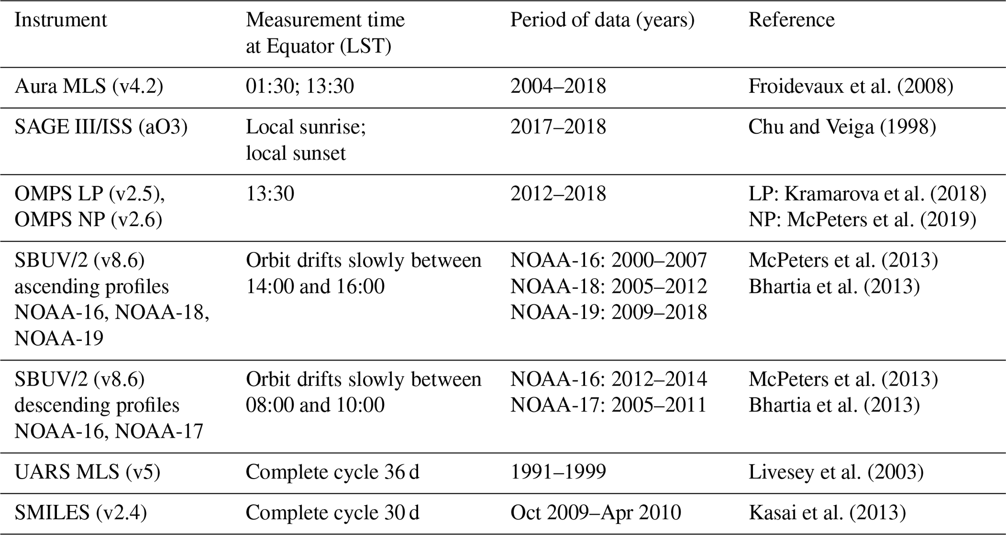
All high vertical resolution data records except SAGE III/ISS and OMPS LP are reported in pressure coordinates and are first interpolated to Z^* pressure levels. SAGE III/ISS and OMPS LP data are reported in altitude coordinates, and MERRA-2 dynamical fields are used to convert between geometric altitude and pressure. OMPS NP and SBUV report ozone as partial column densities (in DU) in pressure layers. Number density and mixing ratio profiles are integrated to give cumulative column densities with pressure, which can be interpolated to repartition the partial columns to match the SBUV/OMPS NP broad vertical sampling. Monthly climatological averages of satellite data are constructed (with the exception of SMILES and SAGE III/ISS, which are averaged over the entire available time period) in 5^∘ latitude bins. UARS MLS and SMILES are additionally averaged into 1 h time bins. An estimated seasonal cycle is removed from the 9 months of SMILES data, as outlined in Sakazaki et al. (2013, Fig. 3), and the data are not binned by month. Although UARS MLS also samples the diurnal cycle over an extended period, the geophysical variability is largely removed in the 9-year average by month and the error bars capture the remaining variability. In this work, we use UARS MLS data for qualitative comparisons only; thus, we do not apply a more rigorous analysis to isolate the diurnal cycle.

3 Evaluation of diurnal climatology

3.1 Characterization of the diurnal cycle in GDOC

We first show several examples of GDOC, highlight some of the salient features and compare generally to past studies. Figure 1 shows GDOC, normalized to the value at midnight, as a function of hour of the day and pressure for four latitude bands and months. The ratio is shown with a contour interval of 0.025 (2.5 %). Figure 1a shows the climatology for March at 15–20^∘ N. Here, the most obvious feature is the low ozone during the day in the lower mesosphere, the well-known mesospheric ozone diurnal cycle (e.g., Pallister and Tuck, 1983). There is very little, if any, variation in the nighttime values at these altitudes. Below 1 hPa, there are variations at the sub-5 % level. Unlike at higher levels, near 2 hPa the diurnal ozone nighttime values decrease by 2.5 % between midnight and early morning and then vary up and down during the day (see also Fig. 4b). Results in this latitude band correspond to previous results shown in Parrish et al. (2014), comparing an earlier version of the model to diurnal variations derived from the microwave radiometer at Mauna Loa. Overall, that study showed differences between the model and data that were generally within 1 %–1.5 %. The largest discrepancy was noted during the winter months in the predawn and early morning hours near 2 hPa, where the microwave instrument showed increasing rather than decreasing ozone (Parrish et al., 2014, Fig. 9). However, SMILES data also suggest that the ozone is decreasing over this period (Fig. 4b; Parrish et al., 2014, Fig. 10). Figure S2 (top panels) shows GDOC at 15–20^∘ N for the additional months of January and June. The predawn and early morning diurnal ozone decrease is larger in January, as was seen by Parrish et al. (2014).

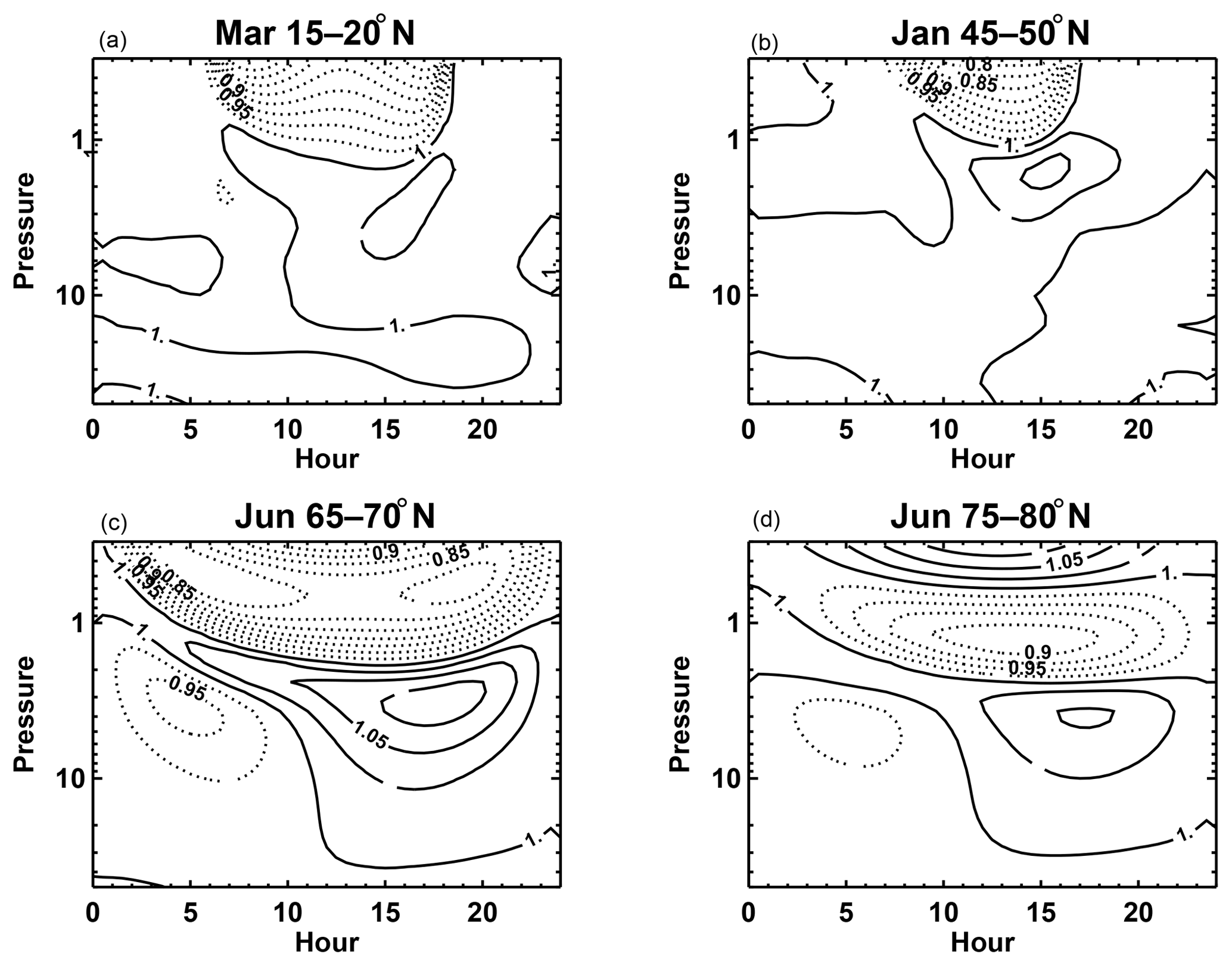
Figure 1 Contour plot of the GEOS-GMI diurnal ozone climatology (GDOC) normalized to the midnight value as a function of hour and pressure for March at 15–20^∘ N (a), January at 45–50^∘ N (b), June at 65–70^∘ N (c) and June at 75–80^∘ N (d). The contour interval is 0.025 (2.5 %). The climatology is shown at levels from 50 to 0.3 hPa.

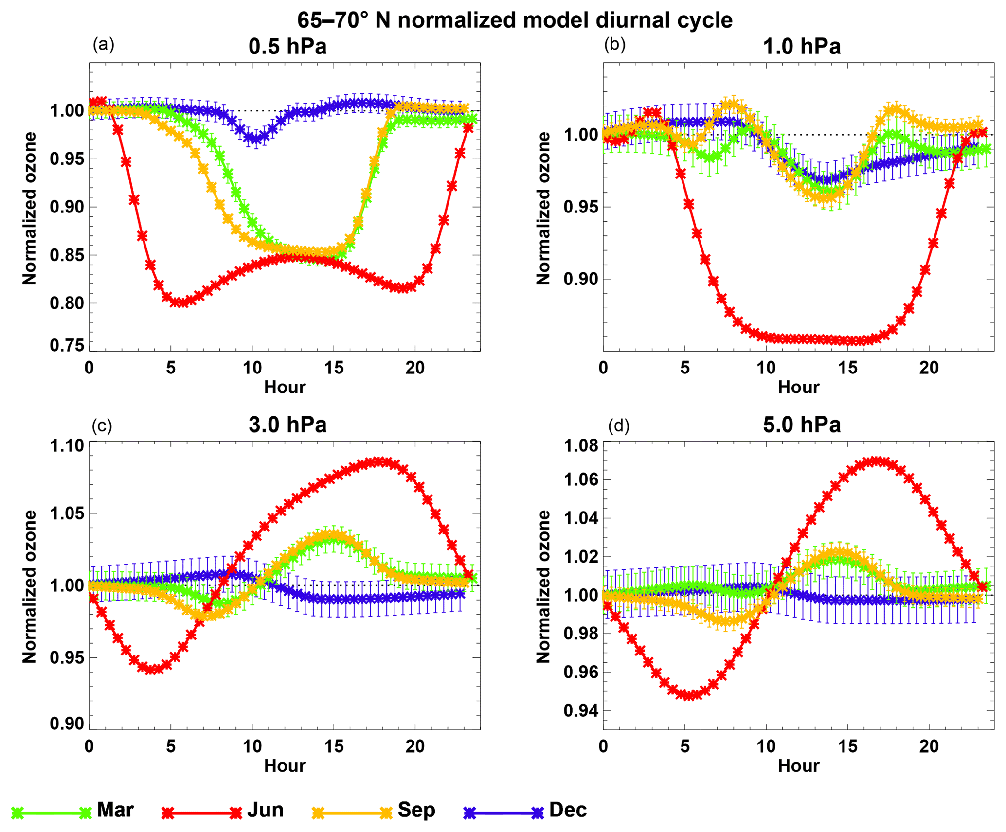
Figure 2 GDOC at 65–70^∘ N as a function of season at four pressure levels: 0.5 hPa (a), 1 hPa (b), 3 hPa (c) and 5 hPa (d). Seasons are represented by monthly output in March, June, September and December. The diurnal signal is plotted as a function of hour (30 min resolution) and is normalized to the midnight value. The error bars are 2SEM, as described in the text. The model uncertainty is largest in winter, when the day-to-day and longitudinal variability of model ozone is greatest.

Figure 1b shows results for January at 45–50^∘ N, which can be directly compared to a diurnal climatology developed from the GROMOS microwave radiometer in Bern, Switzerland (Studer et al., 2014, Fig. 4a), as well as co-located model output from the Whole Atmosphere Community Climate Model (WACCM) and the Hamburg Model of Neutral and Ionized Atmosphere (HAMMONIA) used in the same study. Compared to the March subtropical climatology in Fig. 1a, the shorter period of daylight hours is evident in the higher latitude January output. GDOC shows a loss of just over 20 % at 0.3 hPa, which is somewhat less than that shown by GROMOS or the WACCM and HAMMONIA models, which are closer to 25 %. Below about 1.5 hPa, the pattern shifts from daytime low ozone to a pattern of lower ozone in the morning and higher ozone in the afternoon, with variations of more than 5 %. GROMOS and the co-located models show a similar shift, although at slightly different altitudes. GDOC agrees more closely with the model output from the GROMOS study, and the authors suggest that the limited vertical resolution of the microwave data might be the cause of the discrepancy (Studer et al., 2014). This characteristic pattern with higher afternoon ozone in the upper stratosphere diurnal cycle has been widely reported in other observations from ground-based and satellite data (e.g., Haefele et al., 2008; Huang et al., 2010; Sakazaki et al., 2013; Parrish et al., 2014; Schranz et al., 2018). Using the WACCM model, Schanz et al. (2014a) present a detailed breakdown of the photochemical reactions that contribute to the midlatitude ozone diurnal cycle at 5 hPa (see also Haefele et al., 2008). Figure S3 shows the seasonal variability of GDOC at 45–50^∘ N at several altitudes, which matches the higher summertime amplitude model diurnal cycle reported by Studer et al. (2014) and Schanz et al. (2014a).

Figure 1c and d show the diurnal cycle in the Northern Hemisphere polar summer. The diurnal variability in both the mesosphere and stratosphere is largest near the Arctic Circle (panel c) and decreases nearer the pole (panel d). Near the polar day boundary, the diurnal cycle varies by more than 15 % in the stratosphere. This large signal was reported in WACCM output by Schanz et al. (2014a, b). Recently, 1 year of microwave radiometer data taken at Ny-Ålesund, Spitsbergen, Norway (79^∘ N) showed similar variability with a June peak-to-peak variation of 5 % at 1 hPa (nighttime ozone higher) and similar amplitude variations but with larger afternoon values at 3 hPa (Schranz et al., 2018). The authors also included co-located WACCM model results in their analysis, which compared well with the data after accounting for the reduced vertical resolution of the microwave instrument. The high-resolution WACCM output variations are 10 % at 1 hPa and 8 % at 3 hPa, which is in very close agreement with the GDOC signal at 75–80^∘ S. Figure S2 (bottom panels) shows the summer polar diurnal cycle in the Southern Hemisphere, which is nearly perfectly symmetric with that in the north.

Figure 2 shows GDOC at 65–70^∘ N as a function of time of day at four pressure levels. Climatological values in March, June, September and December demonstrate the marked variation in the diurnal cycle with season at high latitudes. The summertime (June) diurnal cycle is the largest at all pressure levels. At 0.5 hPa (panel a), the square-wave pattern dominates for all seasons, although it is weak in the winter. In the summer, the mesospheric diurnal pattern persists to 1 hPa (panel b), whereas other seasons show a more complicated pattern, with the equinox months showing a secondary peak in the late afternoon. At 3 and 5 hPa (panels c and d), all months except December show an early morning minimum and afternoon maximum. The December diurnal variability is confined to the hours around noon due to limited exposure to sunlight near the polar night boundary. The uncertainty is also greatest in December (winter) at all levels.

A more detailed depiction of the GDOC uncertainty is given in Fig. 3. Here we show the uncertainty at noon local solar time (in percent) as a function of month and latitude at four pressure levels. The uncertainties are very consistent in local solar time, so the noon results are representative of all times. The uncertainties (as defined by the SEM) are mostly less than 1 %. Uncertainties of 1 % or greater, highlighted in red, occur at high latitudes in the winter season of each hemisphere. The largest uncertainties are ∼2 %.

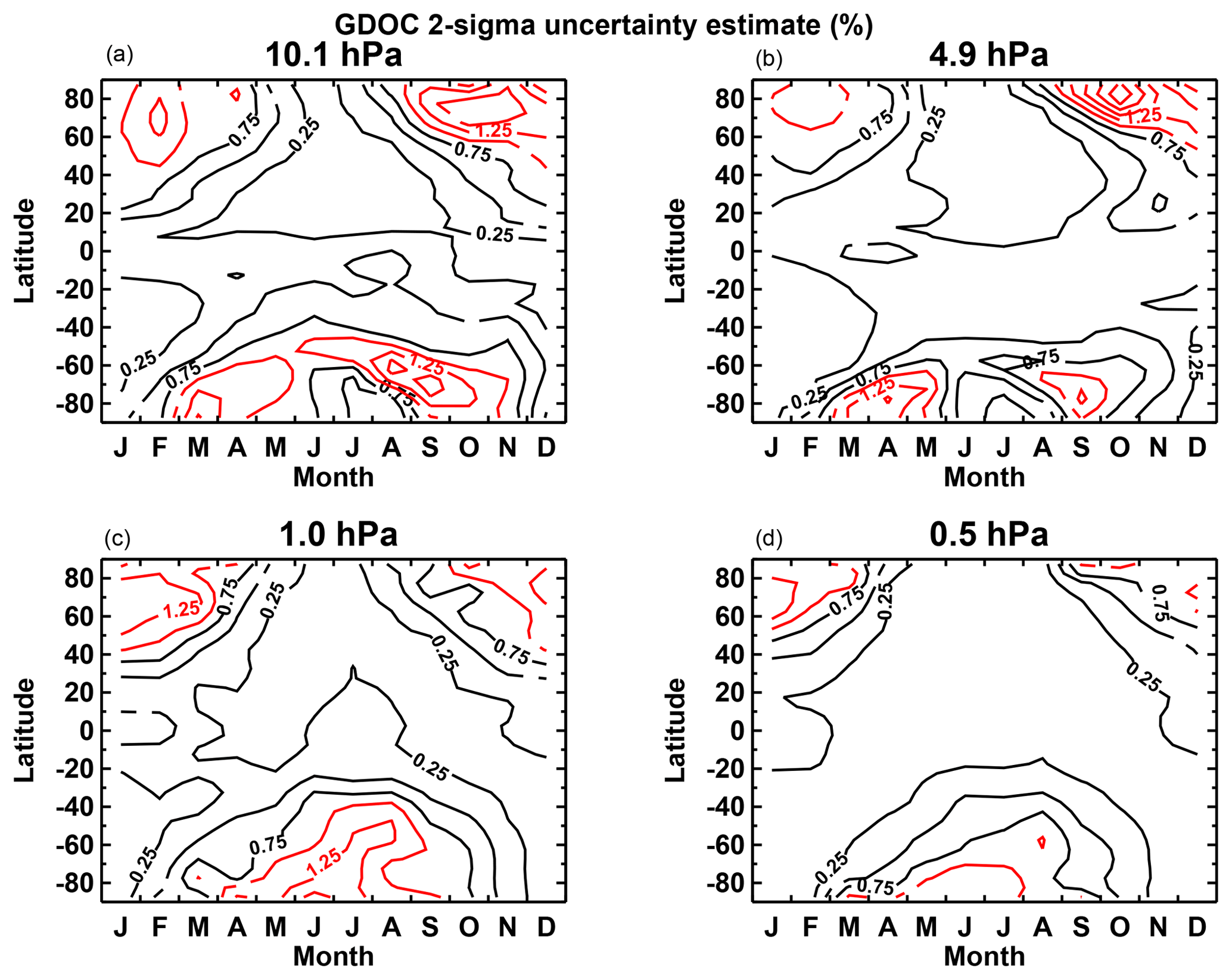
Figure 3 GDOC uncertainty estimates at noon local solar time, plotted as a function of month and latitude at four pressure levels: 10.1 hPa (a), 4.9 hPa (b), 1.0 hPa (c) and 0.5 hPa (d). The uncertainty is defined as the SEM in each bin, which is computed assuming 720 independent data points per bin. Contours of 1 % and greater are highlighted in red.

3.2 Diurnally resolved satellite data

In Fig. 4, we directly compare the general features of GDOC at several pressure levels to those derived from diurnally resolved data from UARS MLS and SMILES satellite-based measurements as well as Aura MLS averages at 01:30 and 13:30 LST (black symbols and vertical dotted lines). Specifically, we plot ozone variability as a function of hour of the day normalized to the mean daily value for each product. The satellite data tend to be noisy, so we normalize to the daily mean rather than to values at a specific time. Because of their orbital characteristics, both UARS MLS and SMILES have their best coverage within ∼30^∘ of the Equator, so we limit our comparisons to low latitudes. We show results at 15–25^∘ N in Fig. 4, but other latitude bands in the tropics are similar. This comparison is qualitative in that we compare the zonal means and we do not attempt to isolate the diurnal cycle in the UARS MLS record beyond simply averaging the data over many years. The deseasonalized SMILES data, as derived in Sakazaki et al. (2013), were provided by the authors (Takatoshi Sakazaki, personal communication, 2014). Although the satellite data are noisy from hour to hour, the overall daily variability is accurately represented by GDOC. At 0.5 hPa (panel a) the mesospheric diurnal pattern prevails, and GDOC captures the amplitude of the day to night ozone differences measured by the satellite instruments. At 1.5 hPa (panel b), the pattern is a hybrid of the mesospheric and stratospheric diurnal cycle, with two relative maxima in the early morning and late afternoon, which is also seen in the SMILES data and, to some degree, by UARS MLS. Finally, at 5 hPa (panel c) the stratospheric pattern dominates, with measurements and climatology showing the highest daily values in the midafternoon. The satellite data agree within ∼4 % on the amplitude of the signal, with GDOC roughly reflecting the average of the satellite data.

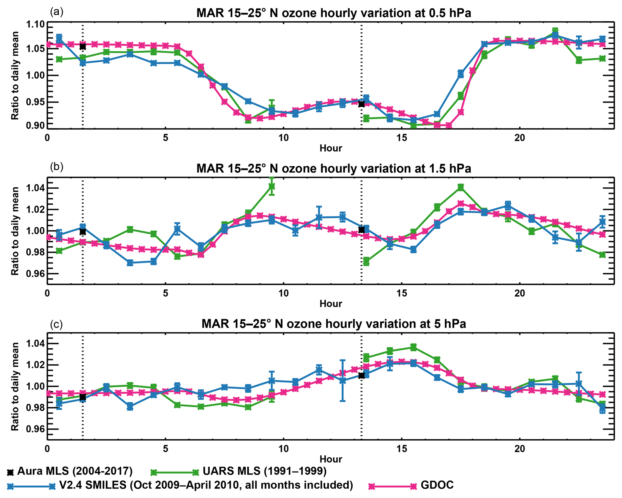
Figure 4 Diurnal variations as derived from SMILES (blue), UARS MLS (green) and Aura MLS (black symbols) compared to GDOC (red), plotted as a function of hour at three pressure levels: 0.5 hPa (a), 1.5 hPa (b) and 5 hPa (c). Each product is normalized by its daily mean value, and the ratio is plotted. The black dotted lines indicate the two daily Aura MLS measurement times. UARS MLS means from 10:00 to 13:00 LST are not computed due to limited sampling. The error bars are 2SEM. For the model and most satellite averages, this error is smaller than the symbol thickness.

3.3 Ascending/descending (day/night) differences

We complete a more rigorous investigation of GDOC by analyzing how well the model reproduces ascending/descending differences in the Aura MLS record. At the Equator, Aura MLS makes measurements at 13:30 and 01:30 LST, but at other latitudes the exact measurement time varies due to the orbit inclination. Outside of polar latitudes, the ascending measurement is made during daylight hours, whereas the descending measurement is made at night. Hereafter we refer to “day” and “night” rather than ascending and descending. Profiles from GDOC are selected to match the location and measurement local solar time of each MLS profile, and they are then averaged for direct comparison with MLS day and night averages. For this comparison, when selecting the climatological profiles, we interpolate in time but not in latitude. Figure 5 shows the ratio of daytime to nighttime averages as measured by Aura MLS (panels a and b) and represented by corresponding profiles from GDOC (panels c and d) as a function of latitude and pressure for 2 months, June and December.

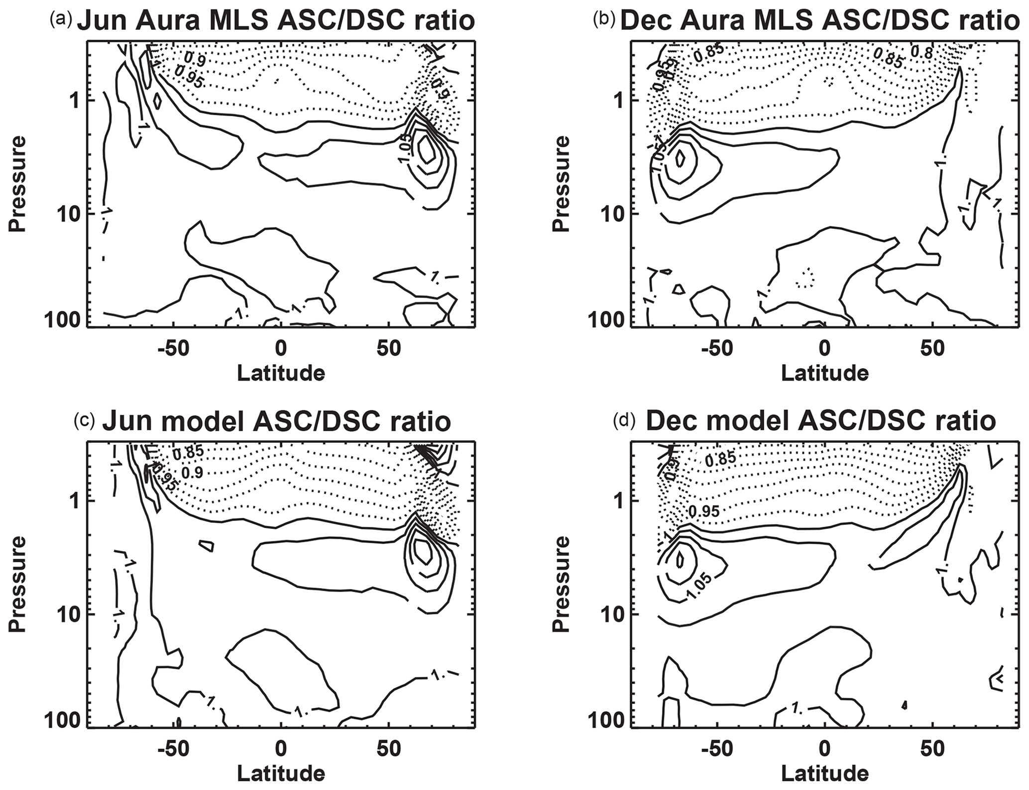
Figure 5 Aura MLS (a, b) and GDOC (c, d) average ratio of ascending (day at most latitudes) to descending (night at most latitudes) average ozone in June (a, c) and December (b, d) as a function of latitude and pressure from 100 to 0.3 hPa. The contour interval is 0.025 (2.5 %). GDOC is sampled at Aura MLS measurement times.

The day to night ratio in the upper stratosphere, above ∼1.5 hPa, shows the typical mesospheric diurnal pattern of low ozone in the daytime and high ozone at night (i.e., Pallister and Tuck, 1983). Below this level the daytime ozone is higher than the nighttime value, but the pattern varies with latitude. As expected, there is little variation between day and night values at high latitudes during polar night (see also Schranz et al., 2018). During polar day, however, there is a variation of greater than 20 % between 5 and 1 hPa near 70^∘ N. Overall GDOC closely matches the spatial pattern and amplitude of the ratios measured by MLS, with agreement generally to within 2 %. In the tropics near 1 hPa, we note a local minimum in the day to night ozone ratio in the Aura MLS data. GDOC also shows a local minimum, but the amplitude of this feature is not as pronounced as in the data. It is interesting to note the similarities in the pattern of the diurnal cycle below 30 hPa. However, we do not validate GDOC below 30 hPa because the diurnal variability is small and does not need to be accounted for at these levels.

Figure 6 shows profiles of the day to night ratio from the model and from Aura MLS at 65–70^∘ N and 65–70^∘ S for the months of March, June, September and December. The error bars indicate twice the standard deviation of the Aura MLS profiles averaged from 2004 to 2018. We show the standard deviation to highlight the interannual variability of the ratio as measured by Aura MLS. In this case, the ratio of the GDOC profiles in the given latitude bin at the ascending and descending time is shown (i.e., GDOC is not explicitly subsampled to each MLS profile), and the error bar is twice the root mean square of the two corresponding uncertainty profiles. Although there are some differences between the model simulations and observations, most notably the small shift in altitude in the June signal at 65–70^∘ N and the offset above 2 hPa in September at 65–70^∘ S, for the most part GDOC reliably reproduces the signal in the observations within 2 % or better. Additional profile comparisons of the day to night ratio from GDOC and Aura MLS can be found in Figs. S4–S9.

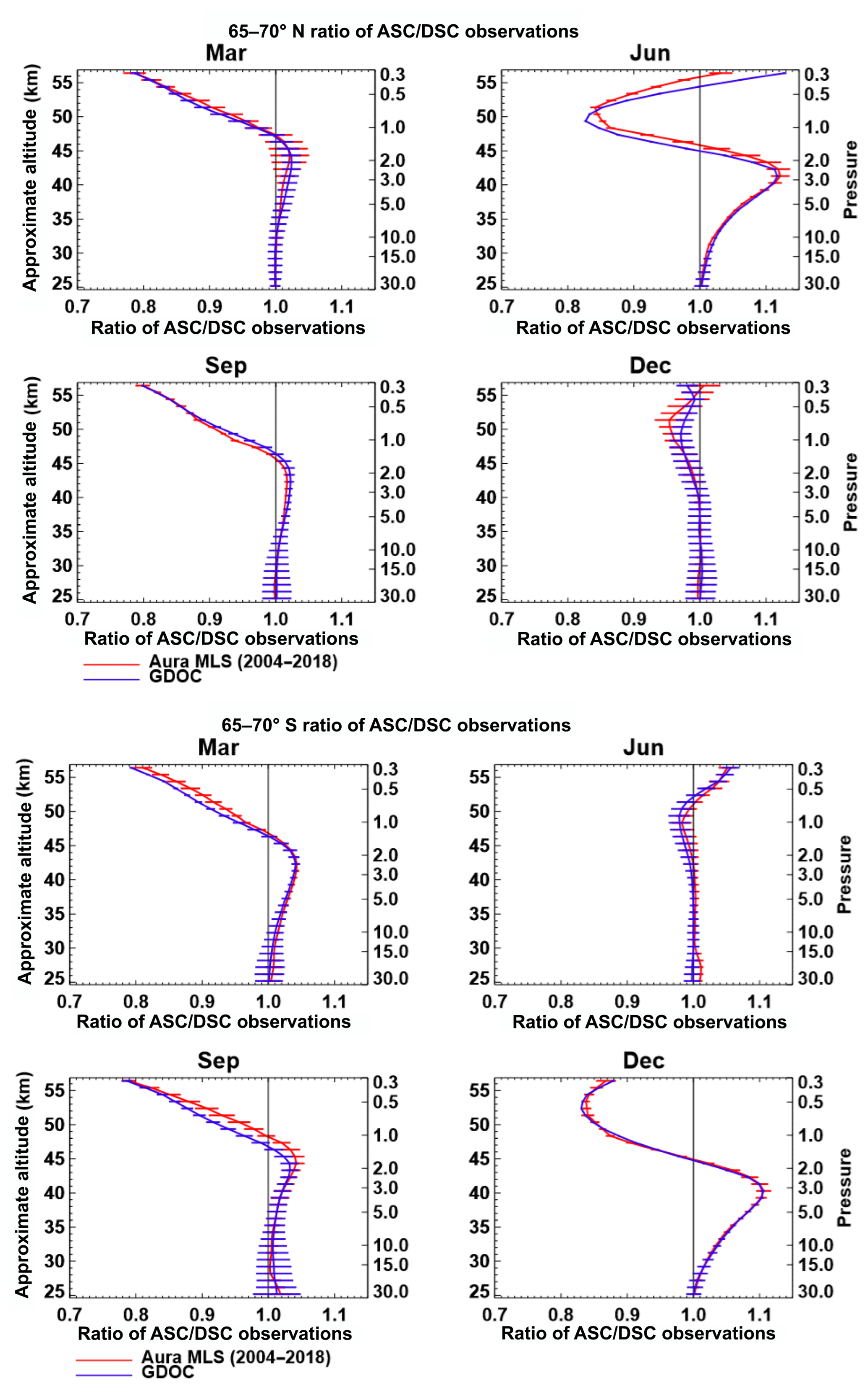
Figure 6 Profile of mean ratio of ascending (day at most latitudes) to descending (night at most latitudes) measurements at 65–70^∘ N (top four panels) and 65–70^∘ S (bottom four panels) from Aura MLS (2004–2018) and GDOC subsampled at Aura MLS profile locations/times. The four panels show results for March, June, September and December. Aura MLS error bars indicate the 2-sigma standard deviation of the Aura MLS ascending/descending ratio profiles from year to year. We show the standard deviation to highlight the interannual variability of the ratio observed by Aura MLS. The model error bars are 2SEM, as described in the text.

4 Example diurnal climatology applications

4.1 SAGE III/ISS sunrise/sunset comparisons

SAGE III/ISS infers ozone profiles by measuring solar irradiance that has passed through the atmosphere during local sunrise and sunset events. One approach to evaluating these data is by checking the consistency of the measured sunrise and sunset profiles, although care must be taken to account for real diurnal differences between sunrise and sunset. Sakazaki et al. (2015) presented a thorough study of sunrise/sunset differences from the SAGE II, UARS HALOE and ACE-FTS occultation instruments in the tropics between 10^∘ N and 10^∘ S. Their analysis included output from the WACCM Specified Dynamics chemical transport model, and both observations and the model indicated an asymmetry between sunrise and sunset measurements in the tropics, with sunrise satellite measurements being larger than those at sunset below ∼30 km and above ∼55 km. Figure 7 shows the ratio of mean (2017–2018) SAGE III/ISS sunrise values to sunset values (SR/SS; red) and the ratio computed from GDOC subsampled to match the SAGE III/ISS measurements (blue). Results are shown in three broad latitude bands, and the SAGE III/ISS profiles have been interpolated to pressure levels (using MERRA-2 temperature/pressure data) in this comparison. The SAGE error bars denote 2SEM, computed as the root mean square of the sunrise and sunset SEM values. The blue error bars for GDOC indicate the variability of the SAGE-sampled reconstructions (computed in the same way as the SAGE error bars). The overlaid orange error bars (roughly the width of the plotting symbol) represents the model uncertainty, computed as the root mean square of the model standard deviation profiles at SAGE sampling, divided by the square root of n (which was set to 720). Note that the spatial–temporal sampling of profiles is different in the sunrise and sunset averages. By matching the diurnal climatology to each profile, we can represent the impact of the sampling on the ratio, but other geophysical variability that the climatology cannot reproduce may contribute to the measured differences. The SR/SS pattern from GDOC is similar to that reported in Sakazaki et al. (2015) with sunrise profiles greater than sunset profiles (ratio >1) below ∼15 hPa (∼30 km) and above ∼0.7 hPa (∼51 km) in the tropics (Fig. 7b). We note that GDOC indicates that $\mathrm{SR}/\mathrm{SS}>\mathrm{1}$ occurs at 51 km, which is somewhat lower than reported by Sakazaki et al. (2015) in observations (∼55 km) and WACCM model results (∼53 km). At midlatitudes, the GDOC sunrise/sunset differences are smaller (SR∕SS is closer to 1), compared with the tropics, with little difference below 15 hPa and a smaller difference in the upper stratosphere. The GDOC SR∕SS pattern is also shifted downward by a few kilometers in the midlatitudes. The SAGE III/ISS SR∕SS ratio generally follows the pattern indicated by GDOC and is within ∼1 % of the GDOC ratio below 2 hPa. Above 2 hPa, GDOC and SAGE III/ISS diverge. At these levels, the SAGE III/ISS retrieval does not account for the sharp diurnal gradient in the ozone along the line of sight of the instrument. However, GDOC representations near the terminator may also be biased due to smearing of the diurnal ozone gradient in the monthly average as the terminator time shifts during the month. Also, as noted above, there is some variation between GDOC, WACCM and observations in the SR∕SS pattern in the tropics. Nevertheless, these differences suggest potential discrepancies between SAGE III/ISS sunrise and sunset measurements that are currently being explored (Robert Damadeo, personal communication, 2019). The purpose of this work is not to evaluate SAGE III/ISS observations but to demonstrate how GDOC can be used in such evaluations.

Figure 7 Ratio of mean sunrise to mean sunset ozone values from the SAGE III/ISS (red) and from GDOC (blue) sampled at SAGE III/ISS profile locations/times from 2017 to 2018. Ratios are shown averaged in broad latitude bands: 20–60^∘ S (a), 20^∘ S to 20^∘ N (b) and 20–60^∘ N (c). The SAGE error bars denote 2SEM, which is computed as the root mean square of the sunrise and sunset SEM values. Note that SAGE III measurements are such that the spatial and temporal sampling are different for the sunrise and sunset mean profiles. The blue error bars for GDOC indicate the variability of the SAGE-sampled reconstructions (computed in the same way as SAGE SEM). The overlaid orange error bars (roughly the width of the plotting symbol) represents the model uncertainty, which is computed as the root mean square of the model standard deviation profiles at SAGE sampling, divided by the square root of n (which was set to 720).

4.2 Comparisons of SAGE III/ISS with other instruments

As with SAGE III/ISS internal sunrise/sunset comparisons, when evaluating the data relative to independent measurements, the local solar time of the measurements should be taken into account. Occultation instruments measure at local sunrise and sunset, whereas limb and nadir measurements are taken at various times throughout the day, depending on the instrument (see Table 1). In this example, we compare SAGE III/ISS sunrise and sunset profiles to co-located profiles from Aura MLS, the OMPS Limb Profiler (OMPS LP) and the OMPS Nadir Profiler (OMPS NP). Both OMPS (LP and NP) and Aura MLS measure at or near 13:30 LST. In the case of Aura MLS and OMPS LP, co-located profiles are defined as the nearest profile (within 1000 km) to the SAGE III/ISS profile, on the same day, and comparisons are done in altitude. Aura MLS profiles are converted from units of volume mixing ratio on pressure surfaces to units of number density on altitude surfaces using co-located MERRA-2 temperature and pressure data. Figure 8 shows mean differences in the 20–60^∘ N latitude band between SAGE III/ISS profiles (sunrise and sunset) relative to OMPS LP (panel a) and Aura MLS (panel b) before (red) and after (blue) using the diurnal climatology to “adjust” the SAGE III/ISS profiles to the equivalent measurement time of the correlative data set. Again, our intention is not to carry out a thorough analysis of the differences but to highlight the influence of the diurnal cycle on such analyses. Near 50 km, the mean differences are reduced by 5 % or more when accounting for the diurnal cycle. Similarly, differences are reduced below 44 km, with SAGE III/ISS coming into very good agreement with Aura MLS at these altitudes.

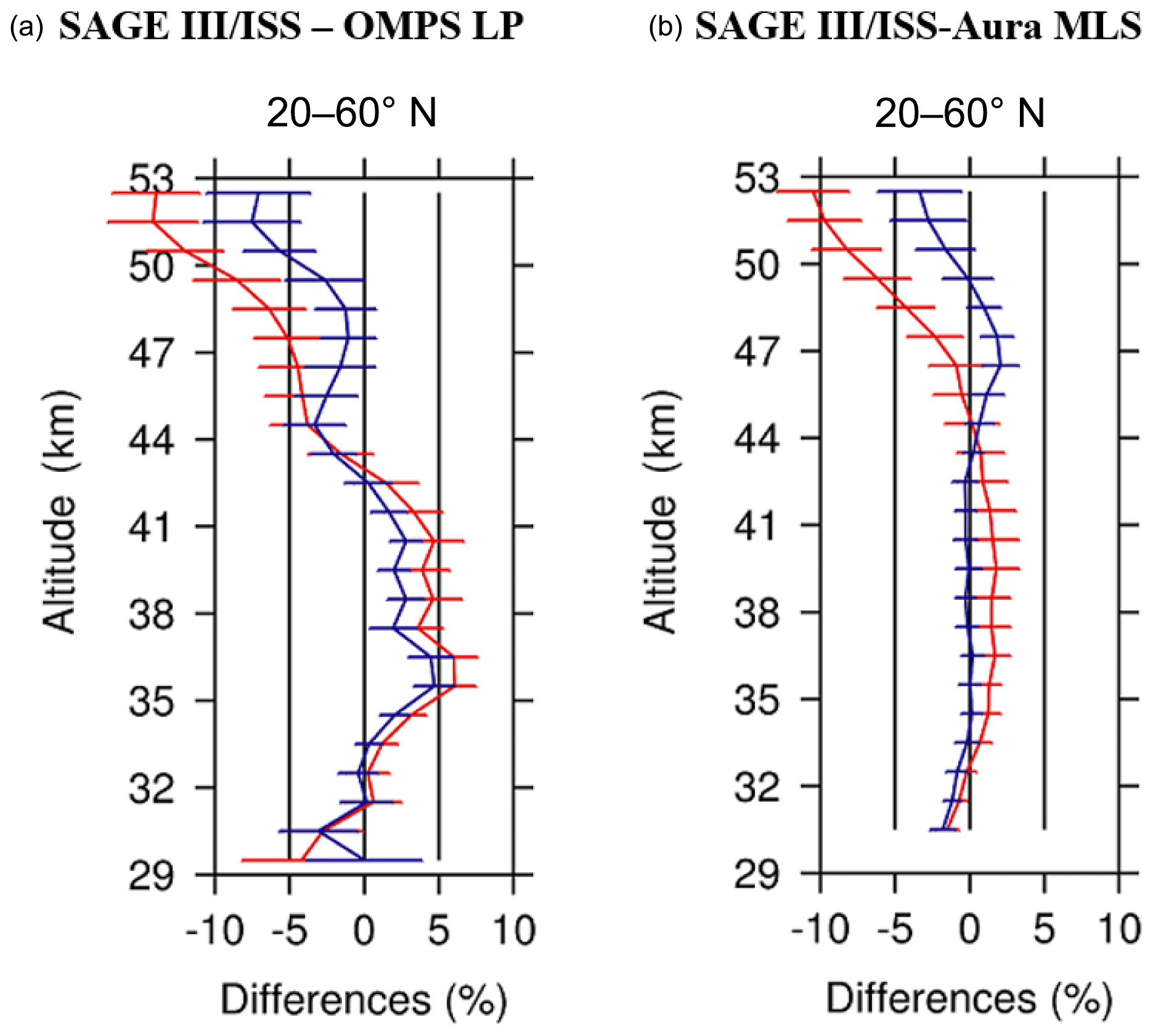
Figure 8 Profile of mean differences between SAGE III/ISS and the OMPS Limb Profiler (a) and Aura MLS (b, daytime measurements only) averaged from 20 to 60^∘ N, expressed as a percentage difference as a function of altitude (km). Sunrise and sunset profiles are included in the mean difference. The red curve shows the original mean difference, and the blue curve shows the same comparison after using GDOC to adjust the SAGE profiles to an equivalent measurement time of 13:30 LST to correspond to OMPS and Aura measurements. The error bars are the standard deviation (1σ; the SEM is smaller than the line width).

Figure 9 shows comparisons between SAGE III/ISS and OMPS NP profiles in three latitude bands. While OMPS LP is a limb scatter instrument that measures at high vertical resolution, OMPS NP is a nadir backscatter measurement with a broad vertical resolution in the stratosphere. Higher resolution instrument measurements (SAGE III/ISS, MLS and OMPS LP) are often used to help evaluate the lower resolution nadir instruments. This is critical to ensure OMPS NP can continue the more than 40-year record of trend quality ozone from the SBUV series of nadir instruments. OMPS NP returns partial column ozone amounts (DU) in pressure layers. Before the SAGE III/ISS sunrise and sunset profiles are averaged, the number density profiles are integrated vertically, giving column densities that are converted to DU and repartitioned into layers that match the OMPS NP vertical resolution. In this case, co-located profiles are the distance-weighted average of all profiles occurring within 1000 km of the SAGE profile on the same day and comparisons are on pressure levels. Figure 9a shows the mean differences for sunrise-only (yellow) and sunset-only (purple) profiles. Figure 9b shows the same differences after the SAGE III/ISS profiles are converted using GDOC to an equivalent time of 13:30 LST to match the time of the OMPS NP measurements. Note that this comparison is focused lower in the stratosphere than in the previous figure. As such, the diurnal impacts are smaller. The largest changes are in the 1.0–1.6 and 1.6–2.5 hPa layers, although there are impacts at the 1 %–2 % level in the 6–10 hPa layer and even lower in the tropics. After the diurnal adjustment, the sunrise and sunset biases are closer, and both indicate a shift in the bias above ∼10 hPa. The remaining pattern of differences is consistent with biases previously reported in the nadir UV backscatter series of instruments relative to satellite (SAGE II, UARS and Aura MLS) and ground-based (select microwave and lidar) data (i.e., Kramarova et al., 2013; Frith et al., 2017). Namely, the nadir backscatter instruments tend to have a negative bias below 10 hPa and above 2.5 hPa and a positive bias near 7 hPa. These examples illustrate how accounting for the diurnal cycle can help to both ascertain the true differences in the profiles and reduce noise in the intercomparisons.

Figure 9 Profile of mean differences between SAGE III/ISS and the OMPS Nadir Profiler (percent difference) as a function of pressure (hPa) separated by SAGE III/ISS sunrise and sunset profiles. Panel (a) shows the original differences, and panel (b) shows the differences after the SAGE III/ISS profiles have been adjusted to the equivalent measurement time of the OMPS NP profiles. The error bars represent 2SEM, based on the month-to-month variability only.

4.3 Merging SBUV ozone records

Representing the diurnal cycle is also important when merging multiple ozone data sets to construct a single long-term consistent data record. In this example, we consider the SBUV series of nadir-view backscatter instruments, which is used to construct the Merged Ozone Data Set (MOD; Frith et al., 2014, 2017). The SBUV/2 instruments on NOAA satellites were launched into drifting orbits such that the measurement time slowly changed over years. In addition, NOAA-17 SBUV/2 was launched into a late morning orbit, whereas the others were in early afternoon orbits, contributing to differences of several hours in overlapping measurements between instruments. Similarly, NOAA-16, although launched into an afternoon orbit, drifted such that measurements after 2012 were made in the early morning.

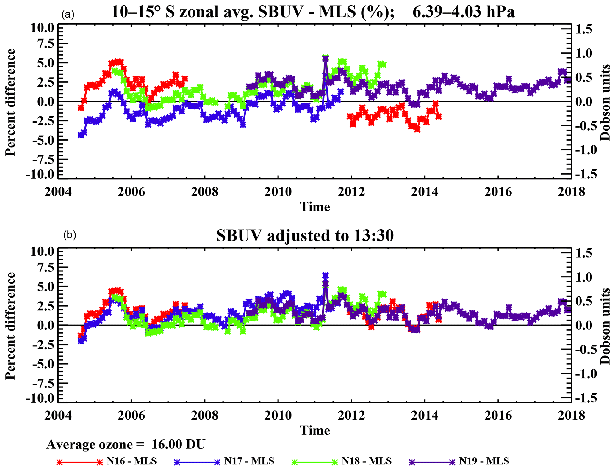
Figure 10 Time series of NOAA-16–NOAA-19 SBUV zonal mean data relative to Aura MLS from 2004 to 2018 in the 10–15^∘ S latitude band and 6–4 hPa pressure layer. Panel (a) shows the original differences, and panel (b) shows the differences after individual SBUV instruments have been adjusted to a common time of 13:30 LST, to coincide with the Aura MLS measurement time. Monthly zonal means of both SBUV and MLS are well sampled such that the uncertainty of 2SEM is smaller than the plot symbols.

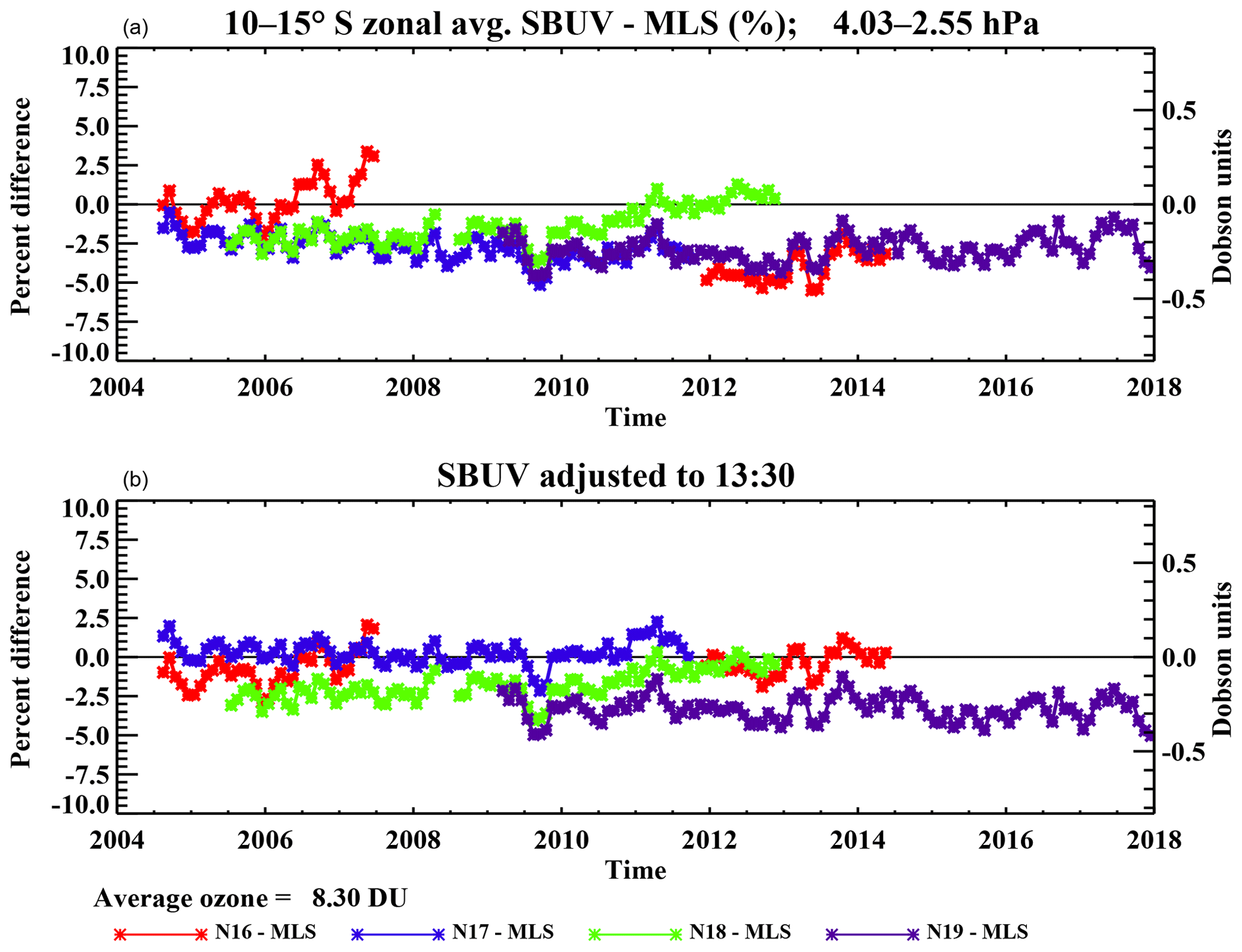
The combination of morning and afternoon orbits and drifting orbits can impart diurnally induced bias, drift and seasonal-scale variation between the SBUV/2 data records. We investigate this by comparing NOAA-16, -17, -18 and -19 to Aura MLS data from 2004 to 2017. Aura MLS volume mixing ratio profiles are integrated to give column density profiles (converted to DU) which are then repartitioned to match the vertical sampling of the SBUV/2 data. Figure 10 shows the 4–6.4 hPa layer ozone difference time series at 10–15^∘ S. Figure 10a shows the original differences between each SBUV/2 instrument and Aura MLS, and Fig. 10b shows the differences after each SBUV measurement has been adjusted using GDOC to the Aura measurement time. Aura MLS is used as a transfer standard and does not change. Here, the primary impact of the diurnal cycle correction is to reduce the bias between the instruments. At the same latitude band but in the 2.5–4 hPa layer, shown in Fig. 11, there are clear drifts over portions of the SBUV records relative to MLS that are largely removed after accounting for the diurnal cycle. Although in this case relative biases between the instruments remain, accounting for a consistent bias in a merged record is much easier than accounting for short-term drifts. Finally, Fig. 12 shows the effect of the seasonal variation in the diurnal cycle at higher latitudes (see Figs. 5 and S3). Here, the SBUV instruments all show a seasonal cycle relative to Aura MLS, but after adjusting for the diurnal cycle the individual SBUV instrument seasonal cycles are in much better agreement relative to MLS. These varied effects can be understood by considering the diurnal cycle in each example, as shown in Fig. S10. The SBUV/2 records shown in Figs. 10–12 vary in measurement time from 14:00 to 16:00 LST and from 08:00 to 10:00 LST. At 10–15^∘ S at 5 hPa there is a difference in the diurnal cycle from morning to afternoon, but little change between 08:00 and 10:00 LST or between 14:00 and 16:00 LST. However at 3 hPa there is a continuous gradient in ozone as a function of hour from 08:00 to 16:00 LST. Thus, there is not only a bias between morning and afternoon measurements, but a drift is also induced as SBUV measurements shift earlier or later in time between the hours of 08:00 to 10:00 LST and 14:00 to 16:00 LST. Finally, at 50–55^∘ S at 7 hPa there is no diurnal signal in June–July–August, but there is a 5 % variation between morning and afternoon ozone in December–January–February, leading to diurnally induced seasonal differences between instruments.

Figure 11 Same as Fig. 10 but for the 10–15^∘ S latitude band at 4–2.5 hPa layer.

Figure 12 Same as Fig. 10 but for the 50–55^∘ S latitude band at 10–6.4 hPa layer.

5 Summary and conclusions

In this paper, we present a global climatology of the ozone diurnal cycle based on the NASA GEOS-GMI chemistry model. The climatology provides ozone values every 30 min during the day, expressed as ratios to the value at midnight (although it can be renormalized relative to other times). It varies as a function of latitude, pressure and month, with a latitude resolution of 5^∘ and a vertical resolution of ∼ 1 km equivalent pressure altitude. Previous studies of diurnal ozone observations often include co-located model results for comparison, but as far as the authors are aware, this is the first easily accessible model-based climatology to be made available for general data analysis purposes. A model-based climatology is useful because no observational data source provides a full representation of the ozone diurnal cycle. However, this fact also makes the model output difficult to validate. Here, we compare the climatology to time-resolved satellite-based data from UARS MLS and SMILES, and compare the day to night climatological ratios to those derived from Aura MLS measurements. We also compare the climatology to previously published results including model analyses and diurnally resolved data from ground-based microwave radiometers. The GEOS-GMI diurnal climatology compares well with all sources; the most quantitative comparison against Aura MLS daytime to nighttime profiles ratios shows agreement typically within 2 %.

The diurnal climatology exhibits the largest variability during summer near the polar day boundary (65–70^∘), as reported previously by Schanz et al. (2014a, b) based on WACCM model output. This is also supported by ratios of daytime to nighttime ozone profiles from Aura MLS. The hourly ozone variation shifts from a mesospheric pattern of low ozone during the day and high ozone at night to a stratospheric pattern of low ozone in the morning and high ozone in the afternoon. However, the amplitude of the signals and the altitude of the transition vary significantly with season, leading to very complicated diurnal patterns that are not easily characterized in data intercomparisons.

In this work, we do not focus on the chemical and dynamical mechanisms of the diurnal cycle but rather on the validity of the model-derived diurnal climatology as a tool for data analysis. We present a series of examples that highlights the usefulness of the climatology in data analysis as well as demonstrates the consistency between the observed and predicted ozone variations. We represent the uncertainty of the climatological mean values as 2SEM of the bin averages, assuming n=720 independent measurements in each bin. This gives error bars that are 2 % or less.

The comparisons presented here give us confidence in the climatology, but we also need to consider potential sources of uncertainty. Systematic changes in the diurnal cycle over a month or from year to year will be smoothed within the climatology. The Aura MLS ASC∕DSC ratios (Figs. 6 and S4–S9) do not suggest significant interannual variability in the large-scale diurnal structure. To further quantify this, we compare GDOC derived using just 2017 model output to that derived using just 2018 model output, as shown in Fig. S11. Below 5 hPa the differences are generally less than 1 %. At higher levels, there are sporadic instances of larger differences (3 %–5 %) in the tropics and at higher latitudes but overall, differences remain small. As more years of model output become available, we will be able to better characterize interannual variability in the model. Similarly, true day-to-day or longitudinal variability in the diurnal cycle will be smoothed out in the zonal average over the month. We find varying degrees of both day-to-day and longitudinal variability in the model diurnal cycles, and this is a subject of ongoing analysis, but characterizing these sources of variability is beyond the scope of this paper. Care should be taken when reconstructing daily values using the monthly GDOC, especially near the terminator in the upper stratosphere, where the ozone gradient is sharp and varies in time over the month.

A final source of uncertainty is potential model error. The climatology is normalized, so the only relevant error is representation of the diurnal cycle. To further test the stability of the model diurnal cycle, we consider several different simulations using iterative versions of the model and/or simulations of different years, and compare the diurnal cycle derived from each simulation. Figure S12 shows the December day–night ratios from diurnal climatologies constructed from four separate simulations. The overall patterns from all the simulations are very similar, suggesting that the representation of the diurnal cycle within the model is well established. This does not preclude a model issue that is present in all model versions. Ideally, as the model is used more in data analyses, such studies will also provide feedback to the modeling team.

We recommend using GDOC primarily for monthly zonal mean analyses in the pressure range from 30 to 0.3 hPa. Comparisons against the various satellite measurements presented in this study suggest that the climatology captures diurnal variations to well within 5 % in most cases. For applications that require accurate knowledge of high temporal and spatial resolution changes in ozone we advise using the original model output (see Sect. “Data availability”).