Evaluation of optical particulate matter sensors under realistic conditions of strong and mild urban pollution

In this paper we evaluate characteristics of three optical particulate matter sensors/sizers (OPS): high-end spectrometer 11-D (Grimm, Germany), low-cost sensor OPC-N2 (Alphasense, United Kingdom) and in-house developed MAQS (Mobile Air Quality System), which is based on another low-cost sensor – PMS5003 (Plantower, China), under realistic conditions of strong and mild urban pollution. Results were compared against a reference gravimetric system, based on a Gemini (Dadolab, Italy), 2.3 m³ h⁻¹ air sampler, with two channels (simultaneously measuring PM_2.5 and PM₁₀ concentrations). The measurements were performed in Sarajevo, the capital of Bosnia-Herzegovina, from December 2019 until May 2020. This interval is divided into period 1 – strong pollution – and period 2 – mild pollution. The city of Sarajevo is one of the most polluted cities in Europe in terms of particulate matter: the average concentration of PM_2.5 during the period 1 was 83 µg m⁻³, with daily average values exceeding 500 µg m⁻³. During period 2, the average concentration of PM_2.5 was 20 µg m⁻³. These conditions represent a good opportunity to test optical devices against the reference instrument in a wide range of ambient particulate matter (PM) concentrations. The effect of an in-house developed diffusion dryer for 11-D is discussed as well. In order to analyse the mass distribution of particles, a scanning mobility particle sizer (SMPS), which together with the 11-D spectrometer gives the full spectrum from nanoparticles of diameter 10 nm to coarse particles of diameter 35 µm, was used. All tested devices showed excellent correlation with the reference instrument in period 1, with R² values between 0.90 and 0.99 for daily average PM concentrations. However, in period 2, where the range of concentrations was much narrower, R² values decreased significantly, to values from 0.28 to 0.92. We have also included results of a 13.5-month long-term comparison of our MAQS sensor with a nearby beta attenuation monitor (BAM) 1020 (Met One Instruments, USA) operated by the United States Environmental Protection Agency (US EPA), which showed similar correlation and no observable change in performance over time.

1 Introduction

Analysis of particulate matter represents a key element for studies of air pollution. Various studies shed light on their effect on health (Downward et al., 2018) and climate (Zhao et al., 2019). In many cases particulate matter is a dominant pollutant among other components of pollution. Therefore, developing a strategy for reliable quantification of particulate matter in ambient air is necessary. The traditional and most accurate approach to measuring the particulate matter concentration in the air is the reference method, based on gravimetric measurements, after the collection of particulate matter by air samplers. The typical time resolution of such measurements is 24 h. Although there are portable air samplers, these measurements are usually performed at fixed locations, such as research supersites. Reference systems are expensive and require a lot of laboratory work. Results are not immediately available because of the time-consuming process of filter treatment. Taking that into account, various governmental institutions usually opt for more affordable and easier-to-use and -maintain equivalent methods. These are usually fixed, semi-automatic stations equipped with beta attenuation monitors (BAMs). The typical time resolution of such stations is 1 h. If maintained and calibrated properly, the equivalent methods should achieve an acceptable level of agreement with the reference. For example, one long-term comprehensive study (Hafkenscheid and Vonk, 2014) performed at 14 different locations across the Netherlands showed that a linear correction $y=\mathrm{0.91}x-\mathrm{1.6}$, applied to raw readings from BAM, was necessary to achieve the requirements of the Guide to the Demonstration of Equivalence (ECWG, 2010).

Newer methods, based on optical particle sensors (OPS), are nowadays increasingly more popular, particularly low-cost variants (Zheng et al., 2019; Mukherjee et al., 2019; Tanzer et al., 2019; Morawska et al., 2018). Their typical time resolution is between 1 s and 1 min, and because of their price and size, they can be used in networks to provide better spatial coverage (Martin et al., 2019; Li et al., 2019). Furthermore, they provide information about multiple mass fractions of particulate matter simultaneously, unlike the concentration of a single fraction in a gravimetric system or BAM. However, there are concerns about their suitability for measuring mass concentrations of ambient PM, since there is a significant measurement uncertainty arising from the principles of their operation.

Most commercially available OPS use Mie scattering theory (Mie, 1908) to determine the size and number of particles within the unit volume of air. Mie theory provides the solution of the Maxwell equations for the scattering of plane waves on spherical particles. The Mie solution is rather complex, but in order to illustrate the non-linearity of the theory, it will suffice to consider the case where particles are much smaller than the wavelength (of light, since a red laser is commonly used in practice). In that case the intensity of scattered radiation is given by

$$\begin{array}{}\text{(1)}& I=I_{\mathrm{0}}{\displaystyle \frac{\mathrm{1}+{\cos }^{\mathrm{2}}\mathit{\theta }}{\mathrm{2}{R}^{\mathrm{2}}}}{\left({\displaystyle \frac{\mathrm{2}\mathit{\pi }}{\mathit{\lambda }}}\right)}^{\mathrm{4}}{\left({\displaystyle \frac{d}{\mathrm{2}}}\right)}^{\mathrm{6}}{\left|{\displaystyle \frac{m^{\mathrm{2}}-\mathrm{1}}{m^{\mathrm{2}}+\mathrm{2}}}\right|}^{\mathrm{2}},\end{array}$$

where I₀ is the intensity of the incident radiation, θ is the scattering angle, R is the distance between the particle and the observing point, λ is the wavelength, d is the particle diameter and m is the refractive index of the particle. Thus, in order to calculate the diameter of the particle by measuring the intensity of the scattered radiation, one must assume a value for the refractive index of the particle. If the particle absorbs nothing from incoming radiation, its refractive index will be real; otherwise, it is written in the form

$$\begin{array}{}\text{(2)}& m=n+i\mathit{\kappa },\end{array}$$

where κ is called the extinction coefficient and is related to the absorption coefficient α:

$$\begin{array}{}\text{(3)}& \mathit{\alpha }={\displaystyle \frac{\mathrm{4}\mathit{\pi }\mathit{\kappa }}{\mathit{\lambda }}}.\end{array}$$

Once the size distribution is calculated across K channels (bins), the total mass concentration of particles will be

$$\begin{array}{}\text{(4)}& c_{\mathrm{m}}=\sum _{i=\mathrm{1}}^K{w}_i{\mathit{\rho }}_i{V}_i{N}_i,\end{array}$$

where V_i is the (average) volume, ρ_i is the density of the particles, N_i is the number of particles per unit volume and w_i is the weighting factor for channel i. Here we have another cause of OPS uncertainty: the density of particles must be assumed. Regarding the weighting factors, sensor manufacturers calculate values to correct for certain effects, such as the fact that OPS cannot detect particles which are too small.

Laboratory tests and calibrations of OPS are performed under controlled conditions with known particles, such as polystyrene latex spheres (Walser et al., 2017; Bezantakos et al., 2018), continuously changing monodisperse particles (Kuula et al., 2017, 2020) or multi-modal particles (Cai et al., 2019). A burning chamber is used in some investigations as well (Wang et al., 2015). However, Eq. (1) is strongly non-linear in terms of refractive index, and in most practical cases corrections for different particles' optical properties are impossible to implement. Furthermore, densities appearing in Eq. (4) are not known a priori. That explains why it is difficult to calibrate OPS for realistic ambient PM concentration measurements: any laboratory calibration may or may not be applicable to the changing outdoor conditions (Tryner et al., 2020; Crilley et al., 2020).

For outdoor applications, there is an additional problem: hygroscopic growth of particles (Jayaratne et al., 2018; Granados-Muñoz et al., 2015; Di Antonio et al., 2018), which leads to overshoots of OPS if the ambient air humidity is (too) high. An obvious solution is to dry the air. However, any proper drying system would cost more than many models of OPS, and it is rarely seen in combination with low-cost sensors. Analytical corrections are often used: humidity sensors are used to measure the relative humidity of ambient air, and some analytical models, like Kohler's theory (Castarède and Thomson, 2018) or the Hänel equation (Hänel, 1976), are applied. Later in this paper we will make some observations on this issue.

Due to all the above-mentioned factors, it is always interesting to check how OPS perform in different realistic scenarios. Numerous papers deal with laboratory calibrations and outdoor evaluations of OPS (Karagulian et al., 2019; Borghi et al., 2018; Chatzidiakou et al., 2019; Magi et al., 2020; Sousan et al., 2016b; Malings et al., 2020; Kelly et al., 2017; Sayahi et al., 2019; Crilley et al., 2018; Zheng et al., 2018; Tasic et al., 2012; Cavaliere et al., 2018; Mukherjee et al., 2017; Sousan et al., 2016a; Zhang et al., 2018; Holstius et al., 2014; Badura et al., 2018). Reported results vary depending on the composition of particulate matter pollution, range of concentrations and meteorological factors. In Mukherjee et al. (2017) OPC-N2, PMS7003 and 11-R were compared against BAM-1020 during 12 weeks in the Cuyama Valley, California, USA. Grimm 11-R performed well, while both OPC-N2 and PMS7003 (which is a miniaturized version of PMS5003) produced mediocre performance with heavy low bias. PurpleAir (PMS5003) was tested in Tryner et al. (2020) using laboratory and field tests. High bias of PMS5003 was observed. In Magi et al. (2020) PurpleAir (PMS5003) was analysed for 16 months in Charlotte, North Carolina, USA, against BAM-1022, and high bias of PMS5003 that increases with humidity was reported. High mean bias of PurpleAir (PMS5003) was reported in Kosmopoulos et al. (2020) as well.

The novelty of this research is a unique combination of instruments and conditions of extremely high urban pollution. The city of Sarajevo is situated in a valley and is affected by strong temperature inversions that appear typically 150–300 m above ground level with a very strong temperature gradient in the inversion layer, exceeding 30 K km⁻¹ (Masic et al., 2019). The inversion episodes were present during most of January 2020. As a consequence, the average monthly concentration of PM_2.5 was very high: 167.3 µg m⁻³. In contrast to that, monthly average values for March and April 2020 were 21.6 and 19.6 µg m⁻³, respectively. This presented an excellent opportunity to test the performance of OPS in very different pollution levels. Simultaneously with OPS and reference gravimetric measurements, a scanning mobility particle sizer (SMPS) was employed to detect nanoparticles. It can detect particles with diameters from 10 nm up to 1 µm. While an SMPS can count very small particles, 11-D can count larger particles, from 0.25 to 35 µm in diameter. When they work simultaneously, they can detect (almost) the full range of particles' diameters, with a span of more than 3 orders of magnitude. This will give detailed insights into the mass distribution of particles.

2 Methodology and experimental setup

The experimental facility was located at the Faculty of Mechanical Engineering in the central part of the Sarajevo valley (43.85424^∘ N, 18.39607^∘ E; 540 m above sea level) and represents well the overall conditions in the city. The reference instrument for measurements of PM concentrations was a Dadolab Gemini air sampler (Fig. 1). It is a single device with two completely independent channels (PM_2.5 and PM₁₀ in this campaign). The filter preparation and gravimetric analysis are performed in a separate laboratory of the Faculty of Science, Department of Chemistry. The air sampler, gravimetric laboratory and all filter procedures satisfied requirements of the standard EN 12341:2014. According to requirements of the standard, all filters were conditioned at relative humidity between 45 % and 50 % and temperature between 19 and 21 ^∘C.

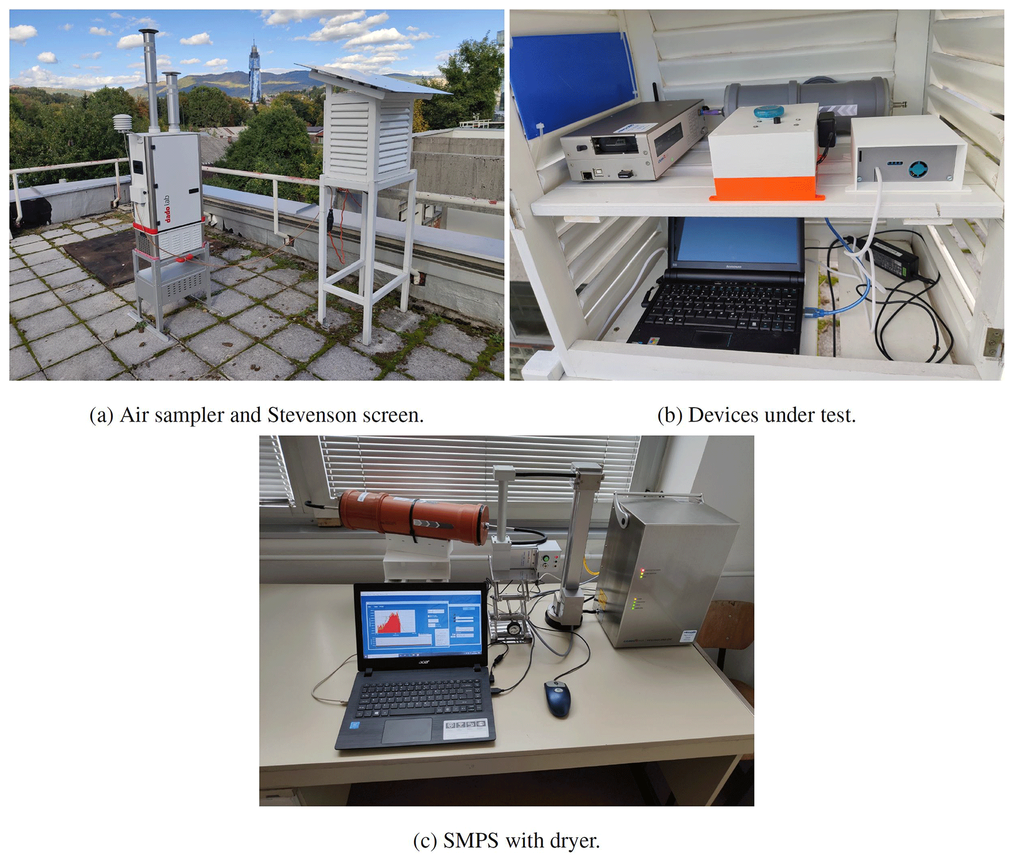
Figure 1 Experimental setup: (a) colocated air sampler and Stevenson screen; (b) devices under test inside of the Stevenson screen: 11-D with dryer, OPC-N2 with SPI adapter and (white-orange) enclosure, MAQS (white enclosure with grey front panel), and (c) indoor SMPS with dryer.

The Grimm 11-D is a high-end optical particle sizer, with sophisticated construction and the ability to count individual particles from 250 nm to 35 µm in 31 equidistant (on logarithmic scale) channels. It uses a proprietary algorithm and the manufacturer does not share information about the refractive index, density or weighting factors. It was factory calibrated and equipped with firmware version 12.50. Data were recorded in 1 min intervals (6 s is also possible). Since we use the common term OPS occasionally, it should be noted that 11-D belongs to a different category of devices (in comparison to low-cost sensors).

Alphasense OPC-N2 belongs to the category of low-cost sensors. The manufacturer transparently shared most specifications. It has a much simpler construction than 11-D: instead of a regulated pump, air flow is provided by a 25 mm fan. The device has 16 channels, from 380 nm to 17 µm. Firmware version 18.2 was used. Refractive index was $n=\mathrm{1.50}+i\mathrm{0}$ and density was 1.65 g cm⁻³. All other parameters, including weighting factors, were used as firmware default values.

Figure 2 AE and SM modes of the PMS5003 sensor.

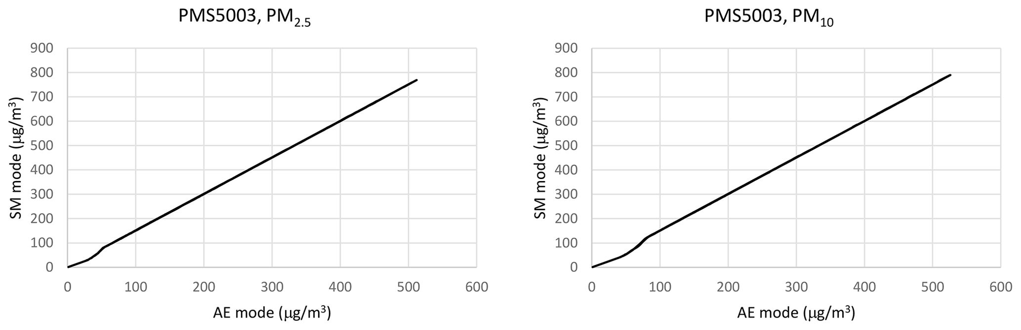
The Plantower PMS5003 could be termed a very low-cost sensor, since its price is lower by an order of magnitude than that of the OPC-N2. Limited specifications do not reveal all operating parameters. From the specification sheet we can conclude that the device uses Mie scattering theory, with a detection limit of 300 nm, and has six channels. It uses a red semiconductor laser, a photodetector at a 90^∘ scattering angle (Kuula et al., 2020) and a 32-bit processor (Cypress CY8C4245, 48 MHz). According to (Tanzer et al., 2019) PMS5003 is a nephelometer, not the particle counter. Air flow is provided by a 20 mm fan. The PMS5003 has two data outputs, one called SM (standard material, CF=1) and another AE (atmospheric environment). The latter mode is used in our work, since the manufacturer recommends the AE mode for ambient air measurements, without further explanation. Figure 2 shows results from our laboratory test using the incense scents as the source of PM. Based on these results, the relationships between the SM and AE modes are

$$\begin{array}{}\text{(5)}& \begin{array}{rl}& {\mathrm{SM}}_{{\mathrm{PM}}_{\mathrm{2.5}}}=\left\{\begin{array}{ll}{\mathrm{AE}}_{{\mathrm{PM}}_{\mathrm{2.5}}}& \text{for }{\mathrm{AE}}_{{\mathrm{PM}}_{\mathrm{2.5}}}\le \mathrm{30}\\ \text{non-linear}& \text{for }\mathrm{30}<{\mathrm{AE}}_{{\mathrm{PM}}_{\mathrm{2.5}}}\le \mathrm{50},\\ \mathrm{1.5}\times {\mathrm{AE}}_{{\mathrm{PM}}_{\mathrm{2.5}}}& \text{for }{\mathrm{AE}}_{{\mathrm{PM}}_{\mathrm{2.5}}}>\mathrm{50}\end{array}\right.\\ & {\mathrm{SM}}_{{\mathrm{PM}}_{\mathrm{10}}}=\left\{\begin{array}{ll}{\mathrm{AE}}_{{\mathrm{PM}}_{\mathrm{10}}}& \text{for }{\mathrm{AE}}_{{\mathrm{PM}}_{\mathrm{10}}}\le \mathrm{43}\\ \text{non-linear}& \text{for }\mathrm{43}<{\mathrm{AE}}_{{\mathrm{PM}}_{\mathrm{10}}}\le \mathrm{77}.\\ \mathrm{1.5}\times {\mathrm{AE}}_{{\mathrm{PM}}_{\mathrm{10}}}& \text{for }{\mathrm{AE}}_{{\mathrm{PM}}_{\mathrm{10}}}>\mathrm{77}\end{array}\right.\end{array}\end{array}$$

Based on PMS5003, we have designed a MAQS (Mobile Air Quality System) smart sensor. Essentially, it is a modular platform for PMS5003, with options for additional sensors (pressure, temperature, humidity, carbon dioxide, wind speed), GNSS receiver, flash memory, WiFi module and 3D-printed enclosure. Eight MAQS sensors were made and tested prior to the main campaign in order to evaluate consistency between units. Figure 3 shows the results of preliminary outdoor measurements for a batch of eight MAQS sensors. They showed very good consistency: the coefficient of determination, R², between any two sensors from the batch was greater than 0.99, and average readings from all sensors are within ±10 % from the average value of the batch of sensors. Data were recorded every minute on a local SD card and remote cloud server simultaneously. The recording interval can be as short as 1 s, but there was no need for that.

Figure 3 Preliminary test of eight MAQS sensors, outdoor measurements.

The Grimm 11-D and Alphasense OPC-N2 could not be used outdoors without shelter, while MAQS has a special case which provides basic protection for outdoor use. Furthermore, a netbook PC was used to record data from the OPC-N2. Outdoor shelter had to be constructed to accommodate 11-D with power supply, OPC-N2 with PC and SPI adapter, and MAQS (for better protection). A Stevenson screen-like wooden structure was designed for that purpose. Another MAQS sensor was used at a remote location, for reasons that will be explained later.

For low-cost sensors (OPC-N2 and MAQS) there was no air dryer or heater, since they are typically used in such conditions. We have designed and constructed a diffusion dryer for application on 11-D, which consists of a porous stainless steel tube surrounded with 1 kg of silica gel. The dryer is compact, 25 cm in length with an 8 cm external diameter, and does not reduce the mobility of the instrument. It was installed only during the period of mild pollution.

Meteorological parameters were measured using the Vantage Pro2 (Davis Instruments, USA) weather station with recording intervals of 15 min.

An SMPS is a complex system which consists of a condensation particle counter (CPC), a differential mobility analyser (DMA) and a charge conditioner (often inadequately called a “neutralizer”). Depending on the characteristics of the DMA, the SMPS can be configured for a certain span of particle diameters. We have used a Grimm 5.416 high-end SMPS with a long DMA which is able to separate particles from 10 to 1000 nm into 129 channels, equidistant on a logarithmic scale. Despite the fact that particles with diameters below 10 nm play an important role in nucleation and growth studies (Tiszenkel et al., 2019), their contribution to the mass budget is negligible. Another (larger) in-house developed diffusion dryer was installed at the inlet of the SMPS. A soft X-ray device was used as the charge conditioner. Scanning mode (alternating upscan and downscan) was used for all measurements. One scan takes about 4 min (8 min for both upscan and downscan). When working in parallel, the SMPS and 11-D form a powerful wide-range spectrometer, which covers a range of particle diameters from 10 nm to 35 µm in 160 channels. Additionally, there is an overlapping area between 250 and 1000 nm where we can see how well these two instruments match. The complex SMPS system was kept indoors (an unavoidable necessity, since both X-ray charger and DMA use very high operating voltages). The air was sampled from outside using a conductive tube of the shortest possible length to avoid particle losses. It was running continuously, except for the periods of maintenance.

A rigorous data validation procedure was used. All instruments were inspected periodically and data logs were analysed thoroughly. When calculating daily average values, complete and consistent data series were required.

3 Results and discussion

During this campaign 296 filters were used in the reference air sampler. After the removal of several blank filters used for periodic verification and those with incomplete sampling (the pneumatic system of the air sampler failed to load new filters automatically a couple of times), 288 filters remained: 143 PM_2.5 and 145 PM₁₀ samples. Figure 2 shows PM_2.5 and PM₁₀ daily average concentrations, together with hourly and daily values of ambient air temperature and relative humidity.

Some modifications of the shelter for 11-D and OPC-N2 were necessary, making those instruments unavailable periodically during December and January. Additionally, more frequent maintenance, such as cleaning of 11-D, was needed when working in extreme conditions. The same goes for the SMPS, which was maintained according to the recommendations of the manufacturer. Taking into account difficult operating conditions, the amount of data collected is satisfactory during the period of strong pollution and excellent during the period of mild pollution. The lower limit of detection (LLoD) of PM_2.5 concentration for evaluated optical aerosol devices is estimated based on their actual field performance. Standard deviation (σ) was calculated for periods with near-zero ambient PM concentration, and an average value of 3σ is the estimated LLoD. For PMS5003 our final estimation is 5 µg m⁻³. The same value is an estimation of Magi et al. (2020), calculated by averaging segmented regressions, and Bulot et al. (2019), by combining results from several previous studies. This method applied to OPC-N2 yields an LLoD of 2 and 1 µg m⁻³ for 11-D. For the reference gravimetric system LLoD was calculated using the blank filters, which were treated in exactly the same way as real samples (except the sampling of particulate matter), and the calculated value of LLoD is 0.7 µg m⁻³. All measurements below LLoD were discarded during the quality assurance phase.

3.1 Strong urban pollution

During the period of strong urban pollution (2 December 2019–12 March 2020), the average value of PM_2.5 concentration was 82.9 µg m⁻³, with minimum daily average value 1.3 µg m⁻³ and maximum value 504.9 µg m⁻³ (Fig. 4). In the same period, the average PM₁₀ concentration was 95.5 µg m⁻³, with minimum value 3.6 µg m⁻³ and maximum value 549.0 µg m⁻³. The ratio of average values of concentrations PM_2.5 ∕ PM₁₀ was 0.87. Very good correlations were observed for all three OPS against the reference instrument (Fig. 5). Such a range of ambient PM concentrations was favourable for achievement of high R² values, but non-linear effects of low-cost sensors were observed too.

Figure 4 Reference PM concentrations with ambient air temperature and humidity.

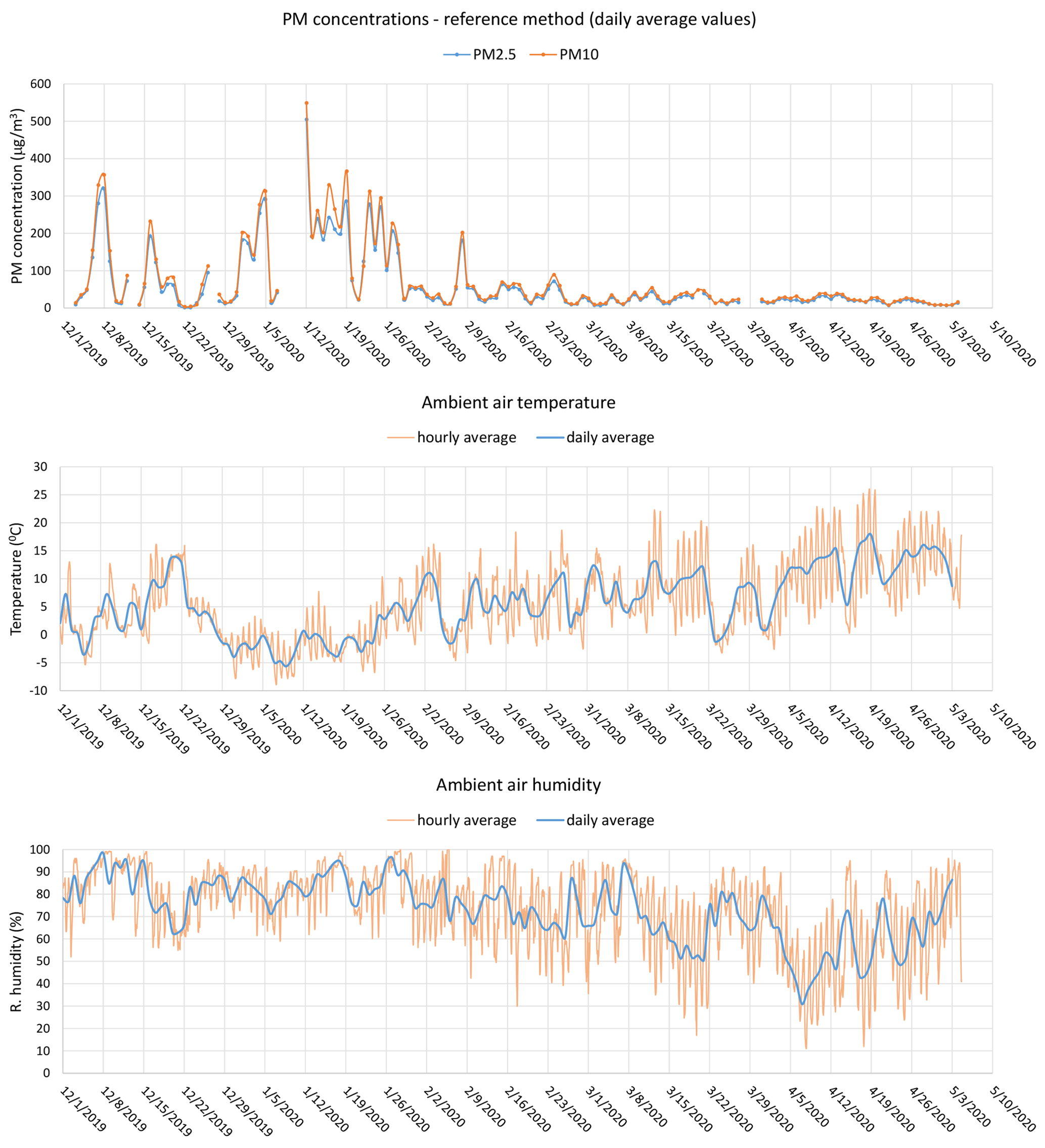
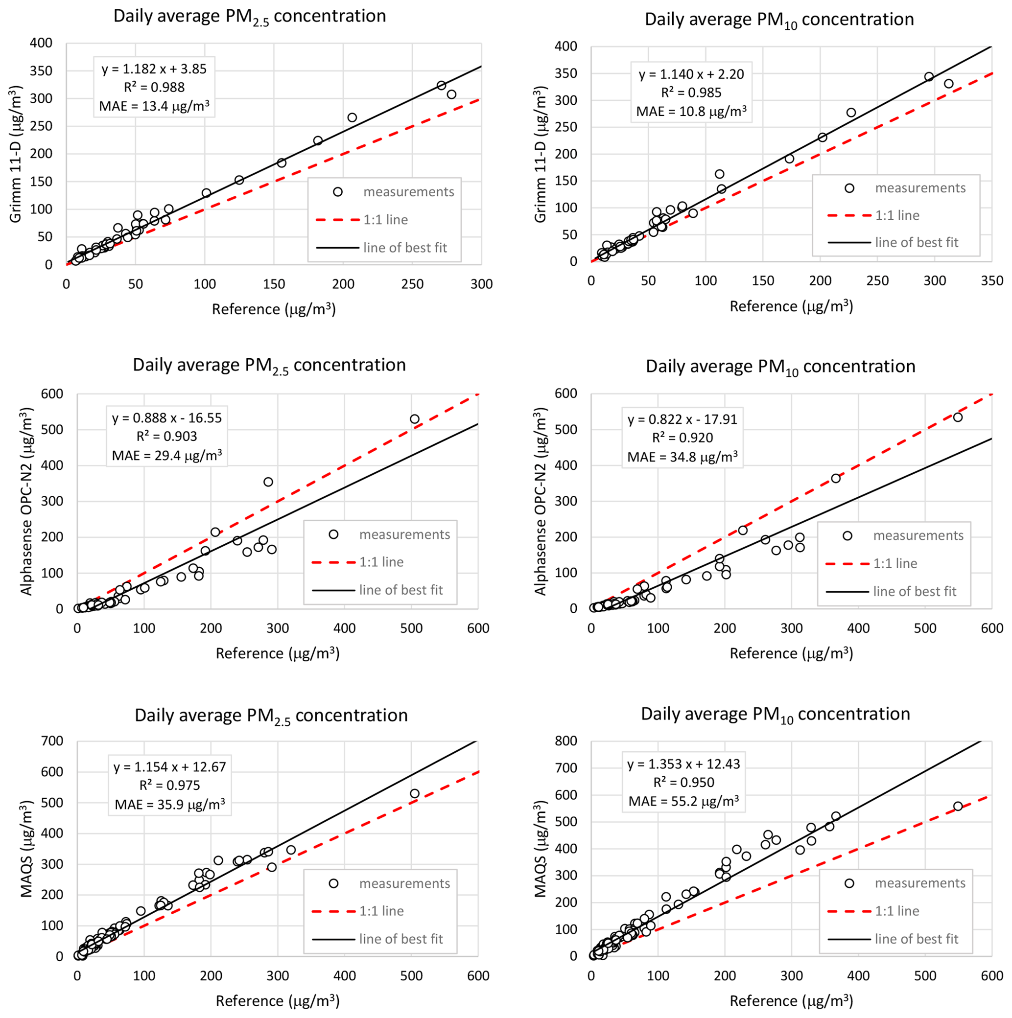
Figure 5 OPS performance during the period of strong pollution (2 December 2019–12 March 2020).

The Grimm 11-D produced results with R² values of 0.988 and 0.985 for PM_2.5 and PM₁₀ concentrations, respectively. Absolute values were larger than the reference, on average 17.6 % for PM_2.5 and 25.5 % for PM₁₀. The average ratio PM_2.5 ∕ PM₁₀ measured by 11-D was 0.93. Mean absolute error (MAE) was 13.4 µg m⁻³ for PM_2.5 and 10.8 µg m⁻³ for PM₁₀. Alphasense OPC-N2 undershoots with respect to the reference values, on average 31.0 % for PM_2.5 and 36.8 % for PM₁₀, but R² coefficients are relatively high: 0.903 and 0.920 for PM_2.5 and PM₁₀, respectively. The OPC-N2 measured the ratio PM_2.5 ∕ PM₁₀ to be 0.97. MAE for this sensor was 29.4 µg m⁻³ for PM_2.5 and 34.8 µg m⁻³ for PM₁₀. The MAQS sensor produced surprisingly good R² values of 0.975 for PM_2.5 and 0.950 for PM₁₀. In terms of absolute values, it overshoots by 31.9 % for PM_2.5 and 49.3 % for PM₁₀ (on average). The calculated ratio PM_2.5 ∕ PM₁₀ was 0.76. MAE was 35.9 µg m⁻³ for PM_2.5 and 55.2 µg m⁻³ for PM₁₀. It seems that the Plantower PMS5003 cannot accurately determine the PM₁₀ fraction. One possible explanation is provided by a laboratory test of PMS5003, where it was found that its size bin [2.5–10 µm] is noisy and inaccurate (Kuula et al., 2020). Further investigation of this behaviour would be useful.

None of the tested OPS were equipped with an air dryer, and this certainly contributes to overprediction. However, Alphasense OPC-N2 with default firmware settings underpredicts values, despite the particle hygroscopic growth effect.

3.2 Mild urban pollution

The correlation coefficients changed dramatically in the period of mild pollution (13 March 2020–4 May 2020), as Fig. 6 shows. The much narrower range of particulate matter concentrations plays an important role, and even the reference method is less accurate, since the mass difference of loaded and blank filters becomes very small (smaller than 1 mg for the 24 h sampling period if PM concentration is below 18 µg m⁻³). The average concentration of PM_2.5 was 19.7 µg m⁻³ with a minimum daily average value of 7.1 µg m⁻³ and a maximum value of 39.3 µg m⁻³. During this period, the average value of the PM₁₀ concentration was 24.2 µg m⁻³, with minimum and maximum values of 7.6 and 48.8 µg m⁻³, respectively. The ratio PM_2.5 ∕ PM₁₀ was 0.81 on average.

Figure 6 OPS performance during the period of mild pollution (13 March 2020–4 May 2020).

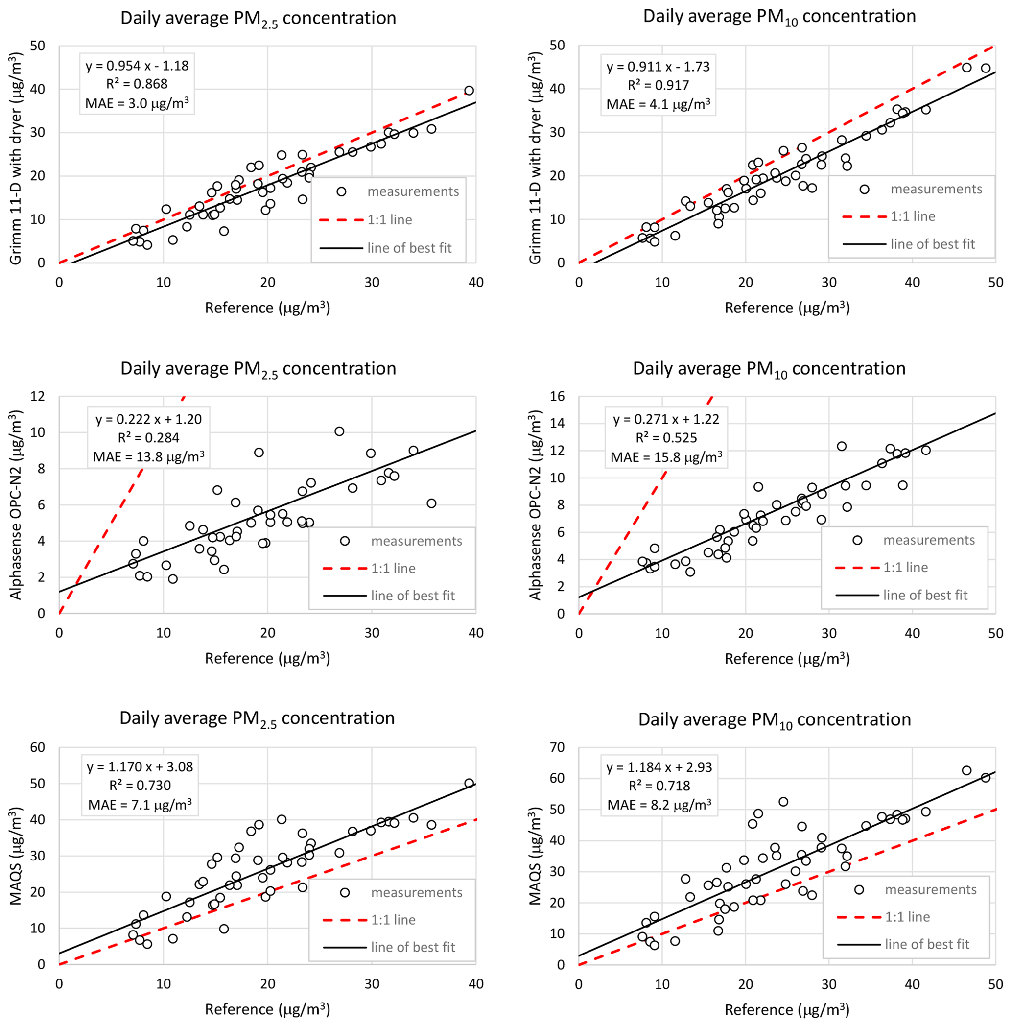
This time the Grimm 11-D was equipped with a dryer, whose effects will be discussed in the next subsection. The device produced relatively high R² values of 0.868 for PM_2.5 and 0.917 for PM₁₀. The absolute readings underestimated concentrations of PM_2.5 by 16.3 % on average, while PM₁₀ were underestimated by 10.9 % on average. The PM_2.5 ∕ PM₁₀ ratio was 0.87. This test clearly shows that 11-D is a completely different class of instrument (in comparison to low-cost sensors). When equipped with a dryer, 11-D shows a level of performance comparable to BAM, at least those reported by Hafkenscheid and Vonk (2014). MAE was 3.0 µg m⁻³ for PM_2.5 and 4.1 µg m⁻³ for PM₁₀.

Alphasense OPC-N2 did not perform well during the period of mild pollution. Coefficients of determination, R², were only 0.284 for PM_2.5 and 0.525 for PM₁₀. Absolute readings are worrying: the OPC-N2 underpredicted PM_2.5 by 67.6 % and PM₁₀ by 71.6 % on average. The ratio PM_2.5 ∕ PM₁₀ was 0.73. MAE was 13.8 µg m⁻³ for PM_2.5 and 15.8 µg m⁻³ for PM₁₀.

The MAQS sensor demonstrated mediocre performance, with R² values of 0.730 for PM_2.5 and 0.718 for PM₁₀. On average, this sensor overpredicted PM_2.5 by 30.5 % and PM₁₀ by 32.6 %. The PM_2.5 ∕ PM₁₀ ratio was 0.83, very close to the reference value (in contrast to the performance of the sensor in the period of strong pollution). MAE was 7.1 µg m⁻³ for PM_2.5 and 8.2 µg m⁻³ for PM₁₀.

It would be interesting to test low-cost sensors with a proper dryer as well, but that combination is rarely seen in practice.

3.3 Humidity influence

One of the important factors in ambient measurements of PM concentrations is humidity, since the particles reflect more light (i.e. appear larger) during measurements due to hygroscopic growth. This can be described using the Hänel equation:

$$\begin{array}{}\text{(6)}& f_{\mathit{\zeta }}\left(\mathrm{RH}\right)={\left({\displaystyle \frac{\mathrm{1}-\mathrm{RH}}{\mathrm{1}-{\mathrm{RH}}_{\mathrm{ref}}}}\right)}^{-\mathit{\gamma }},\end{array}$$

where f_ζ is the enhancement factor for particle property ζ. Here RH represents the relative humidity and RH_ref is a reference relative humidity:

$$\begin{array}{}\text{(7)}& f_{\mathit{\zeta }}\left(\mathrm{RH}\right)={\displaystyle \frac{\mathit{\zeta }\left(\mathrm{RH}\right)}{\mathit{\zeta }\left({\mathrm{RH}}_{\mathrm{ref}}\right)}}.\end{array}$$

It is important to note that the coefficient γ, which is an indicator of the hygroscopicity of particles, depends on the type of particles (and changes whenever the composition of ambient particles is changed).

If we compare results produced by 11-D relative to the reference, during period 1 (without a dryer) and period 2 (with a dryer), we can see that readings of 11-D were reduced by more than 30 %. However, we cannot conclude whether it was the effect of the dryer or the consequence of significantly different ambient conditions. Unfortunately, we have only one 11-D, so we could not measure simultaneously with and without a dryer (that is the reason why we used the instrument with the dryer only in one of the two periods). If we take into account two intervals with similar ambient conditions, with and without a dryer we get the following values: from 27 February 2020 to 12 March 2020 the average ambient concentration of PM_2.5 was 21.1 µg m⁻³, while 11-D (without a dryer) measured 21.5 % more. In the second interval, from 13 March 2020 to 1 April 2020, the ambient concentration was similar, 21.0 µg m⁻³, while 11-D (with a dryer) measured a 1.4 % smaller value. This comparison indicates that the effect of the dryer could be around 23 %. A similar analysis for PM₁₀ concentrations gives an estimate of about 20 % for the dryer effect.

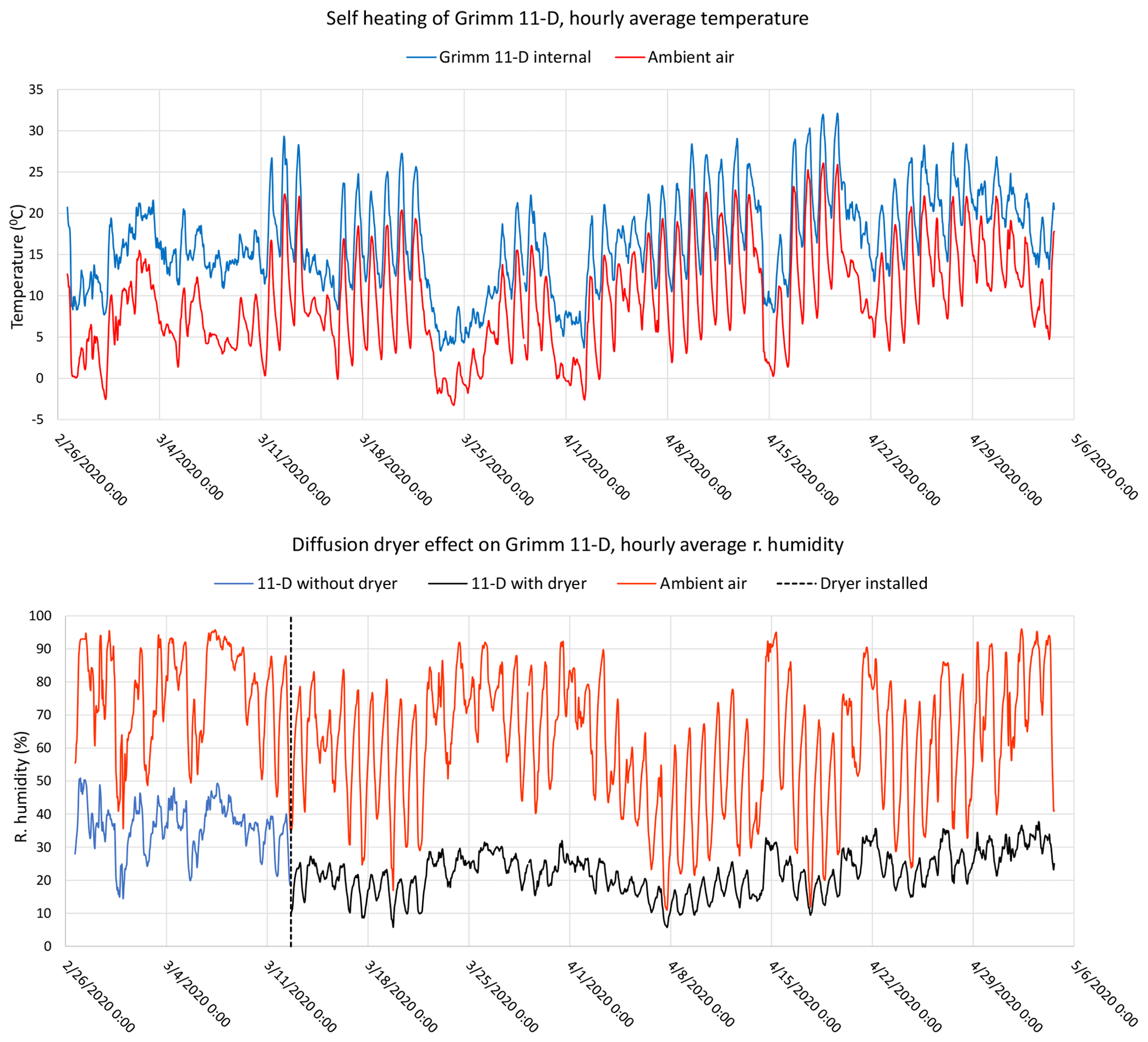
Figure 7 Self-heating and diffusion dryer effect of the Grimm 11-D. The dryer was installed on 12 March 2020 15:30 LT (UTC+1).

The Grimm 11-D has a very useful feature: an internal temperature and humidity sensor. Figure 7 shows the self-heating and diffusion dryer effect on 11-D by comparing internal and external measurements of temperature and humidity. The average ambient air temperature from 27 February 2020 to 1 April 2020 was 7.02 ^∘C, while the average 11-D internal temperature was 14.27 ^∘C, which shows a significant difference of 7.25 ^∘C. This self-heating effect reduces internal humidity significantly, and we can see that it rarely goes beyond 50 %. Once the dryer is installed, internal relative humidity is further reduced: the average value of internal humidity without a dryer (27 February 2020–12 March 2020) was 36.2 %, and with a dryer (13 March 2020–1 April 2020) it was 21.8 % (the ambient air humidity also dropped in the later period, but nevertheless the effect of the dryer is evident).

After roughly a month, the dryer's performance degraded and the silica gel needed a regeneration (but it was not performed since we did not want to interrupt measurements when the end of the campaign was near).

Figure 8 Long-term comparisons of the MAQS sensor with BAM operated by the US EPA at the nearby location: hourly, daily, and monthly average values and comparison of hourly and daily average values of two MAQS sensors: the first one (MAQS) at our main facility and the second one (MAQS-FEE) at the Faculty of Electrical Engineering in the immediate vicinity of BAM-1020.

Figure 8 shows the long-term (13.5-month) comparison of MAQS and BAM-1020 with a time resolution of 1 h, together with measured values of ambient air humidity. By averaging all these data we can estimate the influence of humidity on the MAQS sensor: if we sort the measurements by humidity, a subset of points where humidity is below 50 % has an average bias of 14.3 %, for humidity range 50 %–70 %, bias is 16.5 %, for humidity range 70 %–85 %, bias is 31.6 % and for humidity range 85 %–100 %, bias is 37.3 %. If we subtract the bias of the least humidity subset from the bias of the highest humidity subset, we can estimate that humidity influence adds up to 23 % on PM_2.5 readings from the MAQS sensor, which is a similar result to the analysis of humidity influence on our 11-D with dryer installed. While this influence cannot be neglected, it is still relatively modest. A possible reason is the chemical composition of PM without too many hygroscopic components, but that requires a different type of analysis. A relatively modest humidity influence on PMS5003 was also reported in Jayaratne et al. (2018), and a surprisingly low influence is reported by Kosmopoulos et al. (2020).

3.4 SMPS data and wide-range spectrometer

The wide-range spectrometer (SMPS+11D) produced very valuable results. Figure 9 shows the continuous concentration and mass distributions. It is created from hourly average measurements from the SMPS and 11-D. A relative density of 1.65 was applied in SMPS software (based on LabVIEW) for the mass calculation. No other corrections were performed and all settings were factory defaults. Selected histograms (hourly average values) are shown in Fig. 10. What we can see from Figs. 9 and 10 is that in the period of strong pollution the dominant mass contribution comes from particles with diameters around 300 nm. In terms of concentrations, particles around 100 nm appear in the greatest numbers, with occasional secondary peaks coming from even smaller particles.

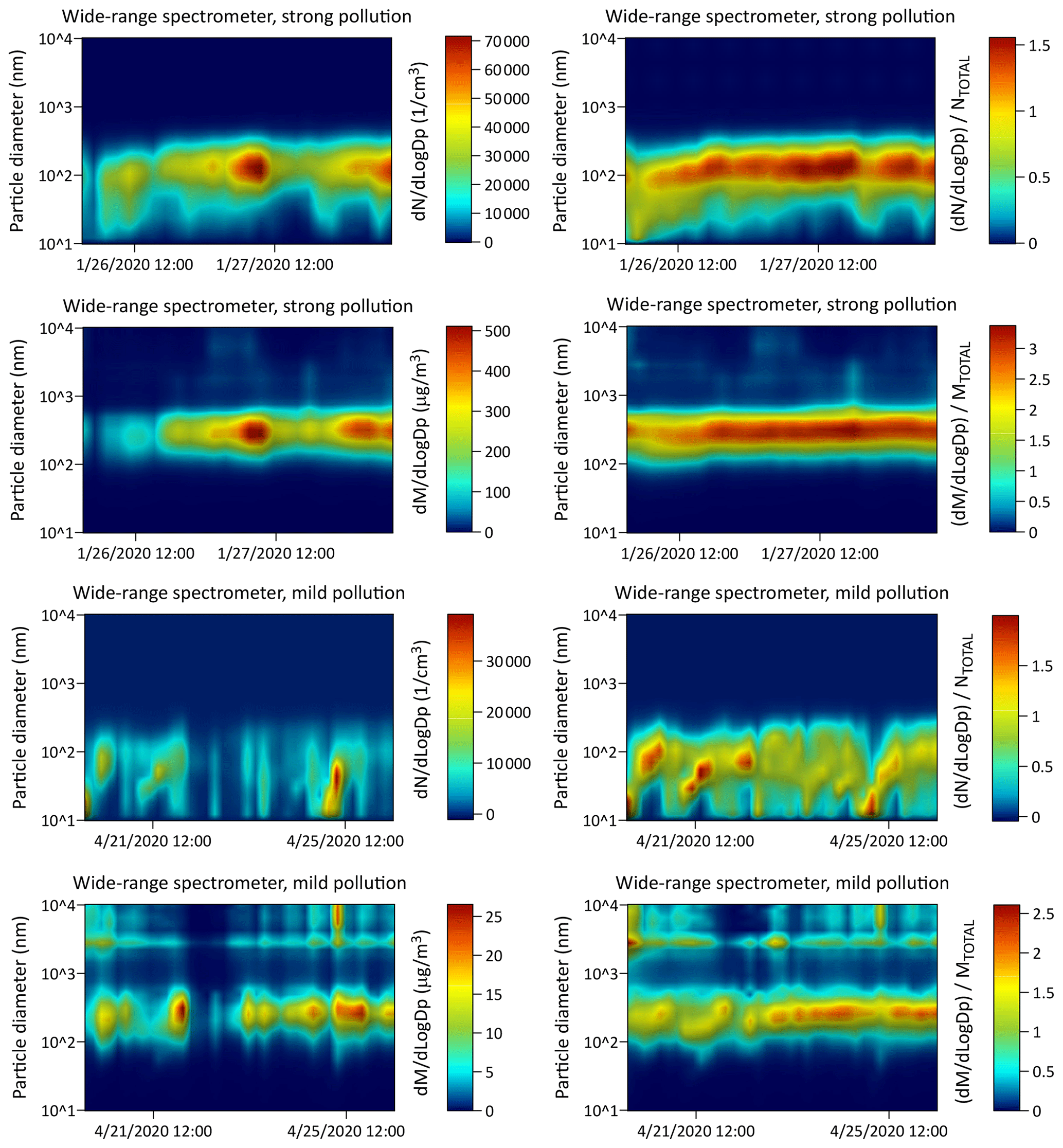
Figure 9 Wide-range spectrometer (SMPS+11D) and hourly average values. Relative density 1.65 was applied to the SMPS to calculate mass of particles.

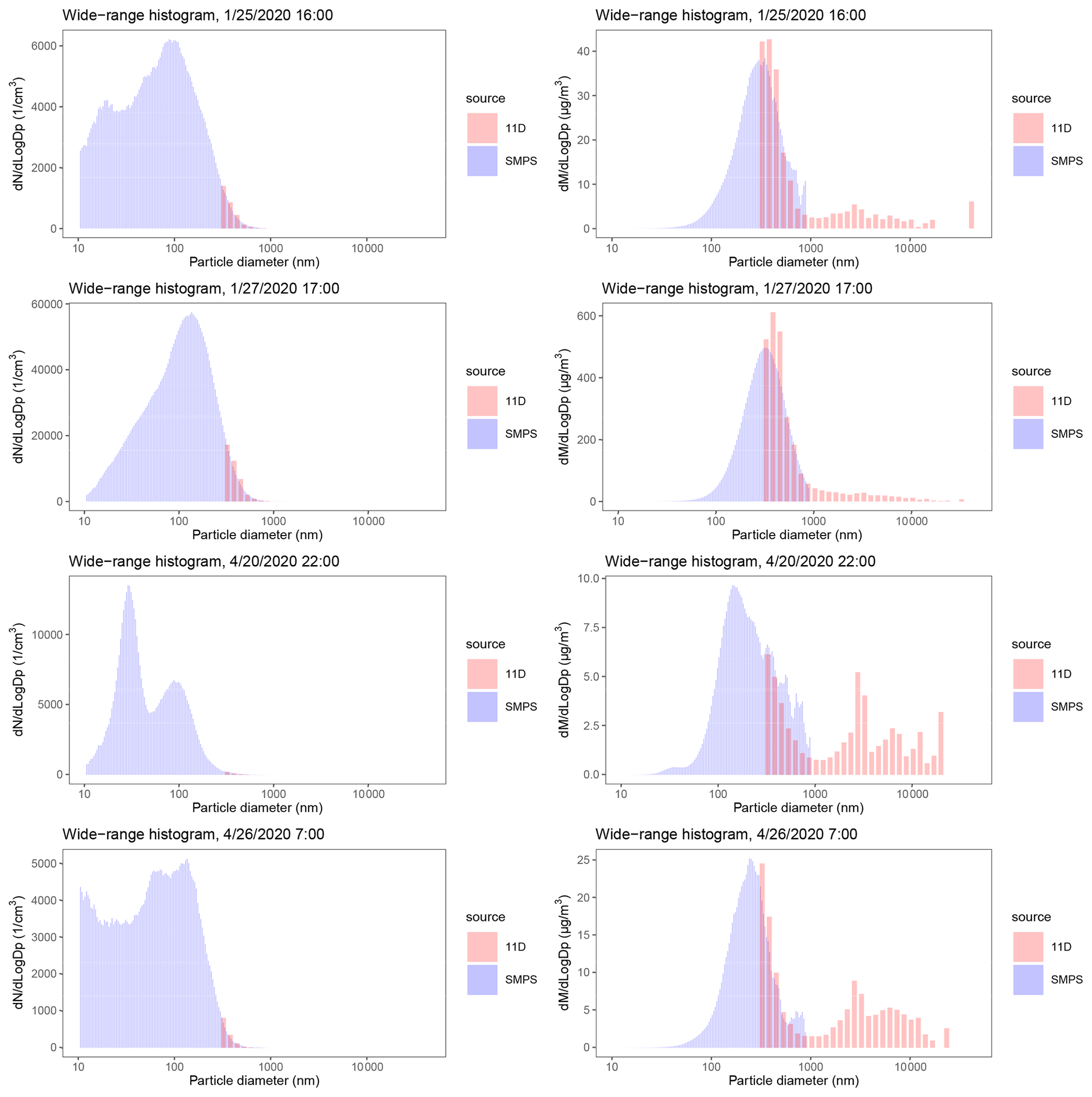
Figure 10 Wide-range histograms and hourly average values. Relative density 1.65 was applied to the SMPS to calculate mass of particles.

In the period of mild pollution, however, we can see that particles larger than 2.5 µm often appear on histograms (usually about 3 µm in diameter). Number concentrations still have peaks of about 100 nm, but sometimes the distribution is different in favour of even smaller particles, as Fig. 10 shows. Again, the largest mass contribution comes from particles around 300 nm.

In the overlapping area, the SMPS and 11-D matched very well, almost perfectly for concentrations. Their match was not as good for mass calculations, but that is understandable, taking into account all the factors explained in Sect. 1. Overall, the combination of the SMPS and 11-D worked very well and gave the full spectrum of particles, both for number concentrations and mass distribution.

The obtained mass distribution of particles, especially during the period of strong pollution, raises the question of the suitability of OPS for measuring mass concentrations and resolving different fractions, since they cannot detect small particles that significantly contribute to the total mass. For example, the Alphasense OPC-N2 has a detection limit of 380 nm and cannot detect the particles around 300 nm which form the dominant contribution to the mass budget. The Grimm 11-D, with a detection limit of 250 nm, has a far better potential to resolve mass fractions.

3.5 OPS histograms and Aralkum Desert dust

All tested OPS have data bins, with different numbers of channels, as described in Sect. 2. Figure 11 shows histograms that compare data bins from 11-D, OPC-N2 and MAQS on 18 January 2020 (strong pollution) and 16 April 2020 (mild pollution). It should be noted that we compare here data bins from devices with different specifications and categories. As expected, 11-D has the ability to count particles below 300 nm, which appear in the greatest numbers. Counting efficiency of OPC-N2 is investigated in laboratory conditions using PSL particles in Sousan et al. (2016a), and the results were good for particles larger than 0.8 µm, while for particles with a diameter of 0.5 µm OPC-N2 the device showed a lower detection efficiency (the detection limit of OPC-N2 is 0.38 µm). In our realistic scenario, the dominant contribution to the mass comes from particles much smaller than 0.8 µm (Figs. 9 and 10), which is not favourable to OPC-N2.

Figure 11 OPS histograms and Aralkum Desert dust episode, hourly average values.

In contrast to OPC-N2, PMS5003 has problems with coarse particles, as indicated in laboratory tests (Kuula et al., 2020). If the fraction of coarse particles is small and steady, PMS5003 performs much better. Ambient conditions in Bosnia-Herzegovina are such most of the time, since the primary source of PM is combustion of coal and biomass. That could explain why PMS5003 performs better than OPC-N2 most of the time. However, different conditions were observed on 27 March 2020, when the dust from the Aralkum Desert covered part of Europe, including our test location. During this episode, OPC-N2 performed much better than PMS5003, which was not able to determine a large fraction of coarse particles correctly (Fig. 11). A similar observation about PMS5003 was reported by Kosmopoulos et al. (2020), when Sahara dust covered Greece.

3.6 Long-term performance

Another question about OPS, especially low-cost types, is the drift of performance over time. The PMS5003 sensor uses a semiconductor laser (diode laser) which has a limited lifetime. We have some long-term comparisons of the MAQS sensor with MetOne BAM-1020 operated at a nearby location by the US EPA. Strictly speaking, their station is not collocated with our equipment, but for a distance of only 300 m it is reasonable to assume that the air composition is very similar at these two points, since they are located in the same neighbourhood. In order to verify that assumption, we have installed another MAQS sensor at the location of the Faculty of Electrical Engineering, University of Sarajevo, which is in the immediate vicinity of the US EPA site and at the same distance from us (about 300 m). Figure 8 shows long-term comparisons of the MAQS sensor and BAM-1020 and additional verification of correlation between readings of the two MAQS sensors, which was very high (R²=0.970, MAE = 4.7 µg m⁻³ for hourly average values and R²=0.994, MAE = 2.9 µg m⁻³ for daily average values), confirming our assumption that these two locations share the same air in terms of PM concentrations and properties.

Based on 13.5 months of continuous comparison of MAQS and BAM-1020, hourly average values give R² coefficient 0.919 and MAE 16.7 µg m⁻³. Daily average values produce R² coefficient 0.980 and MAE 12.2 µg m⁻³, while the monthly average values give R²=0.998 and MAE = 11.4 µg m⁻³ (Fig. 8).

This leads us to the conclusion that time averaging reduces by a lot the influence of variation of PM composition and meteorological variations. If we use a longer time-average period, we lose one of the major advantages of low-cost sensors (time resolution), but it is a more natural approach to correcting readings compared to using artificial algorithms like neural networks (Badura et al., 2019) or machine learning (Si et al., 2020). An excellent viewpoint of this issue is given by Hagler et al. (2018). The calibration of a larger number of low-cost sensors can be simplified if they show similar relative performance (to each other) in the laboratory and field (Sousan et al., 2018). Floating corrections, even physically justifiable interventions, such as the instantaneous correction for humidity growth of particles, insert a lot of noise, and the benefit is questionable. Depending on ambient conditions, self heating of the sensor and some other factors, relative humidity may not be accurately determined. Even if we have a very accurate humidity measurement, the hygroscopic growth coefficient will change whenever the composition of PM changes, inevitably injecting noise into the results.

We can also see strong non-linear effects at very high concentrations, above 500 µg m⁻³. In that case a quadratic regression fit will be more suitable.

During this period of 13.5 months of continuous outdoor operation, the MAQS sensor worked flawlessly without performance drifts. Designed enclosure sufficiently protected the sensor outdoors while not obstructing air sampling.

4 Conclusions

A comprehensive experimental study was carried out with the aim of evaluating the performance of three very different OPS: high-end Grimm 11-D, low-cost Alphasense OPC-N2 and in-house developed MAQS sensor, which is based on another low-cost sensor, the Plantower PMS5003 sensor. The study was performed in realistic conditions of strong and mild urban pollution. The reference instrument was a dual-channel air sampler with gravimetric analysis in a separate laboratory. In total 288 filters were collected from 2 December 2019 to 4 May 2020.

During the period of strong urban pollution all three instruments produced very high R² values. However, during the period of mild urban pollution, these correlation factors dropped significantly, especially for the Alphasense OPC-N2 sensor measuring the PM_2.5 parameter. The OPC-N2 underestimated the mass concentrations badly, especially during the period of mild pollution. The MAQS sensor overshoots PM_2.5 concentrations by approximately 30 % on average, which is partially caused by hygroscopic growth.

The wide-range spectrometer, which consists of the SMPS and 11-D, produced valuable information about the distribution of particles, both in number and mass concentrations. Particles with diameters around 100 nm (and sometimes below) represent the dominant fraction in pure numbers, while particles with diameters of around 300 nm give the highest contribution to mass. In the period of mild pollution, particles larger then 2.5 µm gave a larger contribution than in the period of strong pollution.

The Grimm 11-D performed well in all conditions, and when equipped with a dryer, it performed at a comparable level to the beta attenuation monitor. For the calibration of low-cost sensors, especially those based on PMS5003, we propose a linear or quadratic correction (in the case of high pollution levels) with steady coefficients, since the instantaneous corrections insert noise into results.

Future measurements should further investigate characteristics of OPS in different ambient conditions, influence of humidity and effect of micro-dryers specifically designed for low-cost sensors and mass distributions by means of wide-range spectrometers.