Investigation of three-dimensional radiative transfer effects for UV–Vis satellite and ground-based observations of volcanic plumes

We investigate effects of the three-dimensional (3D) structure of volcanic plumes on the retrieval results of satellite and ground-based UV–Vis observations. For the analysis of such measurements, 1D scenarios are usually assumed (the atmospheric properties only depend on altitude). While 1D assumptions are well suited for the analysis of many atmospheric phenomena, they are usually less appropriate for narrow trace gas plumes. For UV–Vis satellite instruments with large ground pixel sizes like the Global Ozone Monitoring Experiment-2 (GOME-2), the SCanning Imaging Absorption spectroMeter for Atmospheric CHartographY (SCIAMACHY) or the Ozone Monitoring Instrument (OMI), 3D effects are of minor importance, but usually these observations are not sensitive to small volcanic plumes. In contrast, observations of the TROPOspheric Monitoring Instrument (TROPOMI) on board Sentinel-5P have a much smaller ground pixel size (3.5 × 5.5 km²). Thus, on the one hand, TROPOMI can detect much smaller plumes than previous instruments. On the other hand, 3D effects become more important, because the TROPOMI ground pixel size is smaller than the height of the troposphere and also smaller than horizontal atmospheric photon path lengths in the UV–Vis spectral range.

In this study we investigate the following 3D effects using Monte Carlo radiative transfer simulations: (1) the light-mixing effect caused by horizontal photon paths, (2) the saturation effect for strong SO₂ absorption, (3) geometric effects related to slant illumination and viewing angles and (4) plume side-effects related to slant illumination angles and photons reaching the sensor from the sides of volcanic plumes. The first two effects especially can lead to a strong and systematic underestimation of the true trace gas content if 1D retrievals are applied (more than 50 % for the light-mixing effect and up to 100 % for the saturation effect). Besides the atmospheric radiative transfer, the saturation effect also affects the spectral retrievals. Geometric effects have a weaker influence on the quantitative analyses but can lead to a spatial smearing of elevated plumes or even to virtual double plumes. Plume side-effects are small for short wavelengths but can become large for longer wavelengths (up to 100 % for slant viewing and illumination angles). For ground-based observations, most of the above-mentioned 3D effects are not important because of the narrow field of view (FOV) and the closer distance between the instrument and the volcanic plume. However, the light-mixing effect shows a similar strong dependence on the horizontal plume extension as for satellite observations and should be taken into account for the analysis of ground-based observations.

1 Introduction

SO₂ emitted from volcanoes has been observed from satellites for about 40 years. After successful first detections for large eruptions by the TOMS instrument (Krueger, 1983), subsequent UV–Vis satellite instruments with continuous spectral coverage also allowed observation of smaller plume amounts (Eisinger and Burrows, 1998; Afe et al., 2004; Khokhar et al., 2005; Krotkov et al., 2006; Yang et al., 2007, 2010; Nowlan et al., 2011; Rix et al., 2012; Hörmann et al., 2013; Li et al., 2013; Penning de Vries et al., 2014; Theys et al., 2015; Fioletov et al., 2016; Zhang et al., 2017; Theys et al., 2017, 2019, 2021a). Furthermore, besides SO₂, other trace gases like BrO, OClO and IO in volcanic plumes could also be analysed from these observations (Theys et al., 2009; Heue et al., 2011; Rix et al., 2012; Hörmann et al., 2013; Theys et al., 2014; Schönhardt et al., 2017; Suleiman et al., 2019).

Table 1 Ground pixel sizes^a and expected SO₂ SCDs for an SO₂ plume with a horizontal extension smaller than or equal to the size of a TROPOMI pixel and a SO₂ SCD of 1 × 10¹⁶ molec cm⁻² (close to the detection limit) for a GOME-2 observation.

^a For OMI and TROPOMI at nadir. ^b Originally 3.5 × 7 km².

Since the launch of the Global Ozone Monitoring Experiment-1 (GOME-1) instrument on board ERS-2 in 1995 (Burrows et al., 1999), the ground pixel size of UV–Vis sensors has strongly decreased from 40 × 320 km² (GOME-1) down to 3.5 × 5.5 km² (the TROPOspheric Monitoring Instrument – TROPOMI); see Table 1. The ground pixel size of TROPOMI is thus only slightly larger than or even similar to the extension of plumes emitted from point sources, in particular to those from small/medium volcanic eruptions or passive degassing. Thus, with TROPOMI, many small/medium volcanic plumes have become detectable, which could not be detected with the former instruments (the high signal-to-noise ratio of TROPOMI also contributes to the increased sensitivity to small volcanic plumes). An example of TROPOMI observations of SO₂ and BrO for a narrow volcanic plume is shown in Fig. 1 (Warnach, 2022). Shown are the slant column densities (SCDs, commonly interpreted as the integrated concentrations along the light path) of both trace gases.

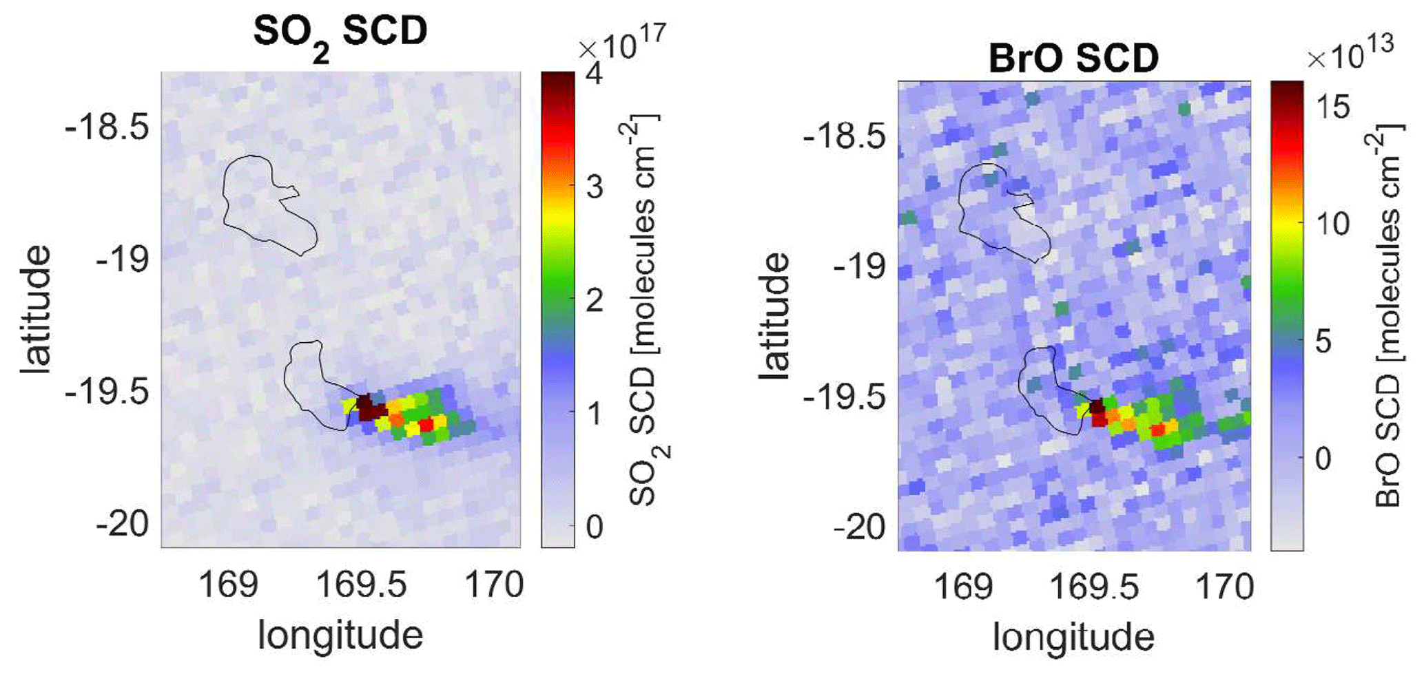
Figure 1 TROPOMI observations of the plume of Mount Yasur on 24 June 2020 (Warnach, 2022).

To illustrate the effects of this improved horizontal resolution, we compare the expected trace gas absorptions of small/medium volcanic plumes for different satellite instruments. As a reference, we take the Global Ozone Monitoring Experiment-2 (GOME-2) instrument, because from GOME-2 observations it was possible for the first time to observe enhanced BrO amounts for several volcanic plumes (Hörmann et al., 2013). A typical detection limit for the SO₂ SCD in the SO₂ standard fit range (about 312 to 324 nm; Hörmann et al., 2013; Theys et al., 2017, 2021b) is about 1 × 10¹⁶ molec cm⁻². The detection limit is similar for the different instruments but depends slightly on the signal-to-noise ratio (see Theys et al., 2019). A SCD of 1 × 10¹⁶ molec cm⁻² corresponds to a differential SO₂ optical depth of about 0.001 when measured with a full width at half maximum (FWHM) of about 0.5 nm, as for TROPOMI. We will use this optical depth as a detection limit for SO₂ in this study. This choice is somewhat arbitrary, but it will serve as a realistic reference point. The detection limit will probably improve in the future using advanced analysis techniques; see e.g. the recent study by Theys et al. (2021a).

If we use the above-mentioned SO₂ SCD of 1 × 10¹⁶ molec cm⁻² for a GOME-2 observation (as a reference case) and assume that the horizontal extension of an observed volcanic plume is smaller than or equal to the size of a TROPOMI ground pixel (e.g. 1 × 1 km² compared to 3.5 × 5.5 km²), we can estimate the SO₂ SCDs observed for instruments with different ground pixel sizes assuming that the measured SCD scales according to the geometric coverage of the volcanic plume. We will see later (light-mixing effect) that assuming simple geometry does not perfectly describe these observations but nevertheless provides a good estimate for the overall effect. The resulting SO₂ SCDs for the different satellite ground pixels are shown in Table 1. The SO₂ SCD for TROPOMI can be higher than the SO₂ SCD for GOME-2 observations by more than 2 orders of magnitude. Even compared to the Ozone Monitoring Instrument (OMI), the increase is larger than a factor of 10.

The results of these simple calculations indicate the great potential of TROPOMI observations for the detection of small/medium volcanic plumes: many weak plumes on the scale of TROPOMI ground pixels were invisible for previous sensors. The corresponding increase in the frequency of detection is difficult to quantify, because the exact frequency distribution of plume sizes and amounts of SO₂ and aerosols is not known. In addition, the self-shielding of plumes by aerosols or clouds formed from the plume probably also depends on the plume sizes themselves. Nevertheless, we can quantify the increase in the detection frequency from the satellite observations themselves. For example, Hörmann et al. (2013) found 220 volcanic SO₂ plumes per year in GOME-2 data, whereas Warnach (2022) found 870 SO₂ plumes per year in TROPOMI data (both studies cover different time periods). In view of the SCD ratios discussed above (see Table 1), this increase by a factor of about 4 in the detection frequency seems rather small (see also Theys et al., 2019). The main and simple reason for the small increase in the number of detections is that many volcanic plumes are larger than the size of a TROPOMI pixel. For such plumes, the SO₂ SCD detected by TROPOMI will be similar to those observed by instruments with larger pixels, up to the size of the plume itself. However, another reason for the rather low increase in detections is related to three-dimensional (3D) effects which are the topic of this paper. As shown below, for TROPOMI observations, 3D effects can cause an underestimation of the true trace gas content of the plume by more than 50 % (light-mixing effect). For plumes with strong SO₂ absorptions, the underestimation can become even larger.

Three-dimensional effects are fundamental effects and do not only affect UV–Vis satellite observations with small ground pixel sizes like TROPOMI. However, for instruments with large ground pixel sizes, 3D effects are typically much smaller than for TROPOMI, and the related errors are typically ignored, because they are smaller than other measurement uncertainties (e.g. related to aerosols or the layer height). For small ground pixel sizes (like for TROPOMI), however, the importance of 3D effects increases for the following reasons.

1. The horizontal pixel dimensions are typically smaller (except for situations with low visibility) than atmospheric photon path lengths (see Table 2). Thus, light scattered horizontally across the borders of the satellite ground pixels becomes important.

2. The horizontal pixel dimensions are smaller than the vertical extent of the troposphere. Thus, geometric effects related to slant illumination and viewing geometry become important.

3. The horizontal pixel dimensions are similar to those of volcanic plumes. Thus, the relative contribution of photons from the sides of the plume increases.

4. One TROPOMI ground pixel might cover the very early part of a volcanic plume, for which the SO₂ concentration can be extremely high. Due to the strong SO₂ absorption, photons will then not penetrate the full plume.

Based on these general aspects, different specific 3D effects can be deduced. In this study we investigate and quantify four specific 3D effects. Two of them (light-mixing effect and geometrical effect) were already investigated by Schwaerzel et al. (2020, 2021) for ground-based and aircraft measurements of NO₂. In this study, we extend these investigations to satellite observations (with different ground pixel sizes). We also investigate two additional 3D effects (saturation effects and plume side-effects). The four specific 3D effects are described in more detail below (see also Fig. 2).

• a.

  Light-mixing effect: part of the detected photons originates from air masses outside the observed ground pixel (and also from outside the trace gas plume). This leads to a reduction in the trace gas absorption compared to the scenario of a horizontally extended plume (Fig. 2a). Here it should be noted that, in the case of spatially varying surface albedo or aerosol distributions, the light-mixing effect could be further enhanced (over a dark surface surrounded by a bright surface) or decreased (over a bright surface surrounded by a dark surface), which is especially important for aerosol retrievals from satellites (Richter, 1990; Lyapustin and Kaufman, 2001). Also, the contributions from different parts within the ground pixel depend on the brightness distribution within the pixel. However, here we focus on scenarios with a constant surface albedo.

• b.

  Saturation effect (Fig. 2b): for strong trace gas absorptions (especially for SO₂ in volcanic plumes), the exact spatial extent of the plume (depending e.g. on the mixing with air from outside) becomes important. If e.g. a trace gas amount is confined to a small part of the satellite ground pixel, the absorption in that part can become very strong. In extreme cases the back-scattered light intensity can even approach zero. Then all light measured by the satellite will originate from the remaining part of the satellite ground pixel (outside the narrow plume), where no SO₂ absorption takes place. In such extreme cases, no trace gas absorption will effectively be observed by the satellite. If instead the same amount of molecules (exact number of molecules) is distributed over a larger volume (and thus a larger fraction of the satellite ground pixel), an increased (but typically still too small) SO₂ absorption will be seen. Thus, the effective trace gas absorption systematically depends on the horizontal extent of a plume and thus on the temporal evolution of the plume and its mixing with air from outside.

• c.

  Geometric effects: for TROPOMI, the ground pixel size is smaller than the vertical extent of the troposphere. Thus, especially for elevated plumes, geometric effects caused by slant viewing directions and/or slant solar illumination angles can cause a smearing-out and apparent displacement of the volcanic plume compared to its true location. In extreme cases, even double plumes might result (Fig. 2c).

• d.

  Plume side-effects: especially if aerosols are present within the plume, edge effects can become important. Their importance increases with decreasing plume size, because a larger fraction of the measured light then reaches the detector from the sides of the plume compared to the top (Fig. 2d). The plume side-effect includes the light-mixing effect but adds the dependence on illumination and viewing angle.

Usually, all four effects occur for satellite observations at the same time. However, in this study we investigate them separately in order to assess their importance for specific measurement scenarios. For these investigations we use the 3D Monte Carlo model TRACY-2 (Wagner et al., 2007; Kern et al., 2010).

Table 2 Free horizontal light paths (e-folding lengths) for different wavelengths and altitudes considering only Rayleigh scattering.

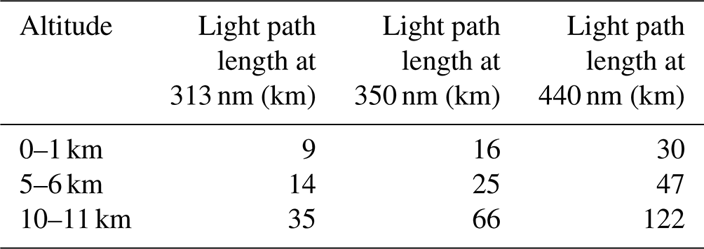
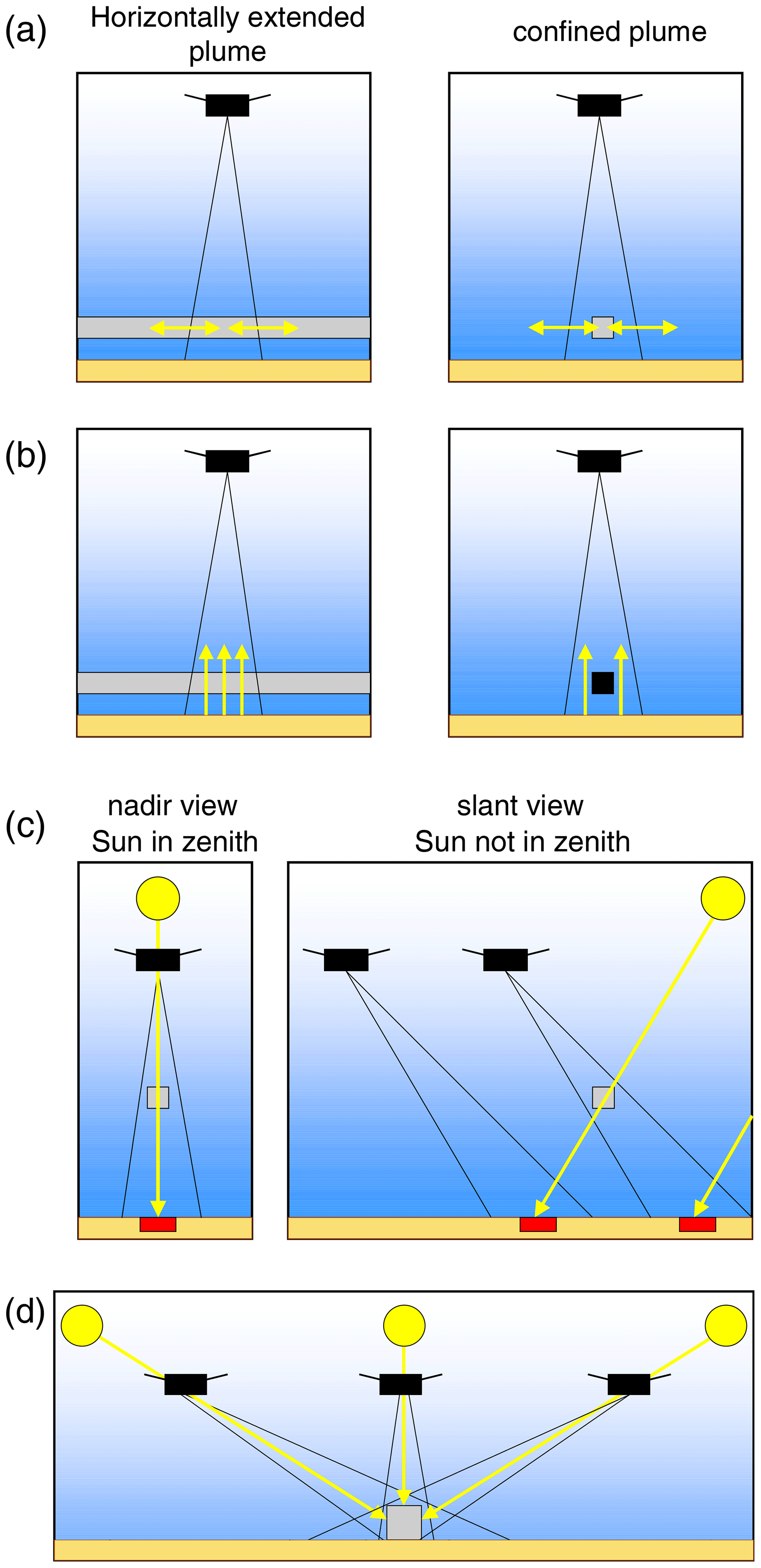
Figure 2 The four 3D effects investigated in this study. (a) Light-mixing effect: part of the light seen by the satellite sensor originates from outside the satellite ground pixel. For horizontally confined plumes (right), such light paths contain no trace gas absorption. (b) Saturation effect: for strongly absorbing species like SO₂, the incoming sunlight might be almost fully absorbed in the plume. This can lead to a strong underestimation for narrow plumes with high trace gas concentrations. (c) Geometric effect: depending on the illumination and viewing geometry, the location of the ground pixel with enhanced trace gas absorption (the projection of the plume along the direction of the incoming sunlight, red marks at the surface, can systematically differ from the true plume location (grey square)). (d) Plume side-effect: for narrow volcanic plumes, the contributions of photons reaching the sensor from the sides of the plume become important.

It should be noted that, for ground-based measurements, a fifth 3D effect becomes important, the so-called light-dilution effect (Kern et al., 2010). It has contributions from the light-mixing effect but is mainly caused by light scattered into the line of sight of the instrument between the plume and the instrument without having crossed the (localised) trace gas plume. Since for satellite observations the observed light typically has not traversed the whole atmosphere, but part of it is scattered above the trace gas layer (leading to air mass factors (AMFs) below unity; for the definition of the AMF, see Sect. 2), the light-dilution effect is already implicitly considered in radiative transfer simulations (even in calculations of 1D AMFs). In this study the light-dilution effect is thus explored as a separate effect only for ground-based observations.

The paper is organised as follows. In Sect. 2 the 3D Monte Carlo radiative transfer model TRACY-2 is introduced. Sections 3 to 6 present simulations of the above-mentioned four 3D effects. Section 7 discusses 3D effects for ground-based observations, and Sect. 8 presents a summary and outlook.

2 The Monte Carlo radiative transfer model TRACY-2

The Monte Carlo radiative transfer model TRACY-2 was developed by Tim Deutschmann at the University of Heidelberg, Germany. TRACY-2 allows the simulation of individual photon paths between the Sun and an observing instrument with flexible boundary conditions. The location and properties of the detector (e.g. width and shape of the field of view, FOV) can be freely chosen. The atmospheric properties, especially the trace gas and aerosol distributions, can be varied in all three dimensions. TRACY-2 is based on the backward Monte Carlo method: a photon emerges from a detector and undergoes various interactions in the atmosphere until the photon leaves the top of the atmosphere (where it is “forced” into the Sun with appropriate weighting factors). A large number of random photon paths is generated, reproducing the light contributing to the simulated measurement. Depending on the atmospheric conditions and the FOV, the number of simulated photons in this study ranges from 10 000 to 1 million. AMFs are derived from the modelled radiances with (I) and without (I₀) the absorber of interest:

$$\begin{array}{}\text{(1)}& \mathrm{AMF}={\displaystyle \frac{\ln \left(I_{\mathrm{0}}/I\right)}{\mathrm{VCD}\cdot \mathit{\sigma }}},\end{array}$$

with σ being the absorption cross section of the considered trace gas and VCD being the vertical column density (the vertically integrated trace gas concentration). Good agreement between TRACY-2 and other radiative transfer models was found in an extensive comparison exercise (Wagner et al., 2007). In Fig. 3 an exemplary simulation with TRACY-2 is shown for a TROPOMI observation of an idealised narrow plume.

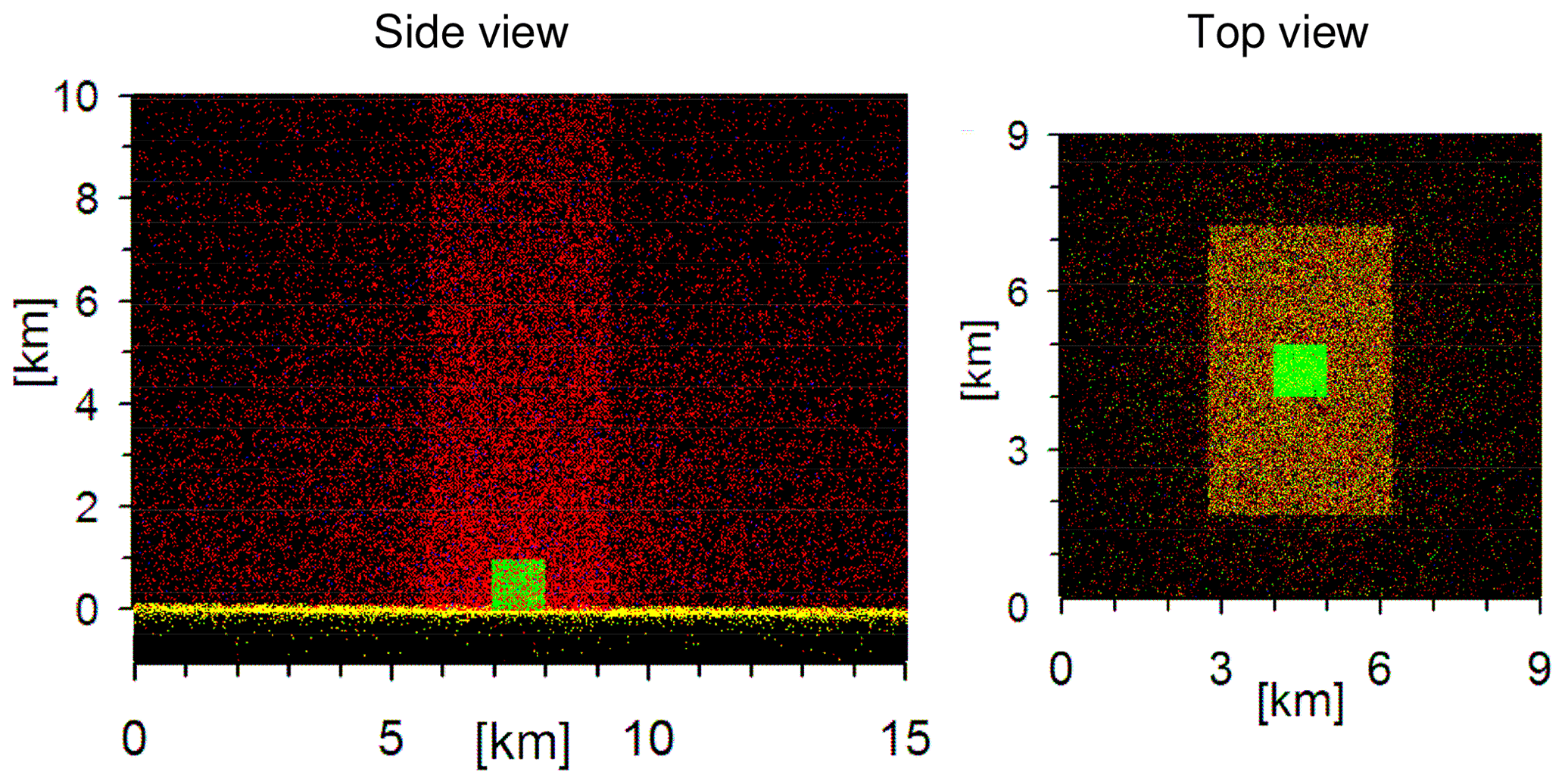
Figure 3 Exemplary simulation results from the Monte Carlo radiative transfer model TRACY-2. An idealised narrow volcanic plume (1 × 1 × 1 km³) is observed by TROPOMI with a FOV according to a ground pixel size of 3.5 × 5.5 km². Red dots indicate Rayleigh scattering events, blue dots rotational Raman scattering events, yellow dots surface reflections and green dots aerosol scattering events (the volcanic plume is filled with purely scattering aerosols). Simulations are performed for 340 nm with 25 000 photons for an overhead Sun and a nadir-viewing satellite instrument.

For the simulations, an atmospheric domain extending ±20^∘ in latitude and longitude around the plume location (centred at 0^∘ longitude and 0^∘ latitude) and from the surface to 1000 km altitude is chosen. The horizontal resolution is high close to the centre (500 m from the centre until 10 km) and coarser outside (11.1 until 111 km, 55.5 until 555 km and one grid cell from 555 to 2222 km). For some simulations (see Figs. 5 and 21), an even finer horizontal grid was used to investigate the effect of very narrow plumes (100 m until 22.5 km, 55.5 until 555 km). The vertical resolution was set to 200 m below 6 km, 1 until 25 km, 2 until 45 km, 5 until 100 km altitude and one layer from 100 to 1000 km. The surface albedo was set to 5 %. This value was chosen because typical albedo values in the considered wavelength ranges over volcanic areas are close to this value (see Fig. A1 in Appendix A). The exact choice of the surface albedo is, nevertheless, not critical, because the ratio of AMFs for narrow plumes and those for horizontally extended plumes hardly depends on the surface albedo (see Fig. A2 in Appendix A). Vertical profiles of temperature, pressure and O₃ concentration are taken from the U.S. Standard Atmosphere (United States Committee on Extension to the Standard Atmosphere, 1976).

The satellite instrument is placed at 824 km above sea level, representing the altitude of TROPOMI. For the investigation of the effects of very narrow plumes (Figs. 5 and 21) and for the plume scans (like in Fig. 6), a narrow FOV of 0.014^∘ (corresponding to a ground pixel diameter of 200 m) is used. For the simulations of real satellite measurements, rectangular FOVs corresponding to the nominal ground pixel sizes of the different satellite instruments (see Table 1) are used.

Volcanic plumes are defined for SO₂, BrO and IO based on ground-based and satellite observations (for details, see Sect. 2.1). Simulations are performed for selected wavelengths relevant to the considered trace gases: for SO₂, four wavelengths (313.1, 324.15, 332.0, 370.3 nm) are chosen for the dominant absorption bands of the different fit ranges (Theys et al., 2017). Simulations for BrO are performed at 340 nm and for IO (and NO₂ and H₂O) at 440 nm. Note that substantial amounts of NO₂ are not expected in volcanic plumes. Also, the increase in the atmospheric water vapour absorption due to water vapour inside the volcanic plume is expected to be very small. Nevertheless, because NO₂ and H₂O are often analysed in the same spectral range as IO, the IO results are also representative of H₂O and NO₂ observations if the ratios of the respective differential cross sections in the spectral range around 440 nm are applied (see Sect. 2.1.3 and Appendix B). Thus, the IO results could also be used for the potential detection of enhanced NO₂ or H₂O in volcanic (or other emission) plumes.

AMFs are calculated according to Eq. (1) for single wavelengths (“monochromatic AMFs”). Thus, the wavelength dependence of the AMF (Marquardt et al., 2000; Puķīte et al., 2010; Puķīte and Wagner, 2016) is not explicitly taken into account, which for strong absorbers usually causes an overestimation of the monochromatic AMFs compared to the true AMFs. In a case study (Sect. 4.3), the effect of the wavelength dependence of the AMF was investigated. It was found that the wavelength dependence of the AMF is negligible for most scenarios (with weak absorptions) considered here. Only for scenarios with strong SO₂ absorptions (with optical depths larger than 0.05 to 0.1) does the wavelength dependence of the AMF become important and further amplify the underestimation of the true AMF. However, such scenarios can easily be identified and excluded from the data analysis, and for such scenarios wavelengths with weaker SO₂ absorptions should be selected. Thus, the effect of the wavelength dependence of the AMF is ignored in this study, and the main findings can be derived from monochromatic AMFs (Eq. 1). While this strongly reduces the computational effort, the computation time for the 3D simulations still remains rather high. The calculation of a single monochromatic 3D AMF takes about 5 min on a state-of-the-art notebook.

2.1 Selected trace gas scenarios

The construction of realistic trace gas scenarios is a challenging task. The assumed trace gas plumes should represent realistic distributions, which are based on ground-based observations. They should also fit satellite observations of narrow plumes, which, however, are often close to the detection limit, because the plumes only cover part of the satellite ground pixel. From the satellite observations no information on the sub-ground pixel scale can be obtained.

For this study, trace gas scenarios were set up for SO₂, BrO and IO. BrO and IO are typically weak absorbers with absorption optical depths clearly below 0.1. Thus, they do not significantly affect the atmospheric light path distribution, and only the relative spatial distribution, not the absolute trace gas amount, is important for the calculation of the AMFs. The scenarios for SO₂, BrO and IO were chosen, because these trace gases were already observed in volcanic plumes. Moreover, the corresponding wavelengths cover the spectral range from about 310 to 440 nm, over which the probability of Rayleigh scattering strongly changes (by a factor of 4). Thus, the light-mixing effect (and also the geometric effect and the side-scattering effect) are expected to differ substantially for the chosen wavelengths. A second set of wavelengths is selected for the SO₂ scenarios (four wavelengths covering the spectral range from about 313 to 370 nm; for details, see Sect. 2.14). However, here we are not primarily interested in the effect of the wavelength dependence of Rayleigh scattering but rather in the strong wavelength dependence of the SO₂ absorption cross section. This second set of wavelengths is used to study the saturation effect for SO₂.

The trace gas scenarios defined below will be used to decide whether the trace gas absorption of a given measurement scenario will be above the detection limit or not. For that purpose we also chose the following detection limits: optical depths of 0.0005 for BrO and IO and 0.001 for SO₂. Of course these choices are somewhat arbitrary but represent realistic reference points for single observations. Here it should be noted that in some cases (e.g. for continuous degassing volcanoes and stable wind fields) many observations might be averaged. In such cases the detection limits will decrease for the statistical mean. Also, for possibly improved future algorithms and instruments, the detection limit might be reduced. Then, observations with trace gas absorptions currently below the detection limit will also become significant, leading to a larger total number of significant observations. Thus, the results obtained in this study should be seen as a general orientation. The differential cross sections (high-frequency amplitudes) used to convert the SCDs of the different trace gases into optical depths are given in Table B1 in Appendix B. Here it should be noted that in our radiative transfer simulations the absolute absorption cross sections were used.

2.1.1 Sizes of the volcanic plumes

Plume diameters close to volcanic vents are typically ≤ 1 km (see e.g. Bobrowski et al., 2003; Bobrowski and Platt, 2007; Dinger et al., 2021). Thus, we assume as a standard scenario a plume with an extension of 1 × 1 × 1 km³. Of course this is a simplification, since realistic plumes close to the volcanic vent will be more complex (including e.g. a vertical updraft above the vent and a horizontal outflow part). However, here we are interested in the basic effects. In addition to the standard scenario, we also assume plumes with larger horizontal extensions but with the same vertical extent and the same total amount of molecules. This allows us to study the light-mixing effect and saturation effect depending on the turbulent dilution state of the plume. For simplicity we assume that the dilution will only occur in the horizontal dimensions. For most simulations (light-mixing effect and saturation effect) we investigate plumes in four altitude ranges: 0–1, 5–6, 10–11 and 15–16 km. For the study of the geometric effects and the side-scattering effects, only plumes at specific heights are chosen to illustrate the general dependencies.

2.1.2 BrO

Maximum BrO SCDs measured from the ground range up to 1.4 × 10¹⁵ molec cm⁻² (Bobrowski et al., 2003; Bobrowski and Platt, 2007; Bobrowski and Giuffrida, 2012). However, because of the sparseness of these observations, the maximum occurring BrO SCDs will probably be higher, and we use in the following a maximum VCD of 5 × 10¹⁵ molec cm⁻² (for the “standard plume” of 1 × 1 × 1 km³). Here we assume that the measured SCD is similar to the corresponding VCD. This assumption is approximately fulfilled for ground-based measurements in the zenith direction or if the plume has an almost circular cross section. Applying simple geometric consideration, this results in a VCD of 2.6 × 10¹⁴ molec cm⁻² for a TROPOMI observation with a ground pixel size of 3.5 × 5.5 km². This value is similar to maximum BrO VCDs observed by TROPOMI for narrow plumes (plumes with extensions of a TROPOMI ground pixel or less). For such cases, Warnach (2022) observed BrO VCDs of up to about 2.5 × 10¹⁴ molec cm⁻² (assuming a 1D AMF of 0.5 corresponding to plumes close to the surface). The BrO scenario corresponds to a total number of BrO molecules in the standard plume (1 × 1 × 1 km³) of 5 × 10²⁵. An overview of the corresponding BrO VCDs for the different horizontal plume extensions is given in Table 3.

Table 3 Plume extensions and corresponding trace gas VCDs and AODs (lowest row) used in this study. For a given scenario the amount of trace gas is assumed to be constant but is distributed over different plume volumes (depending on the horizontal plume extension). The trace gas VCDs of the scenarios with 1 × 1 km² horizontal extension is used to identify the corresponding scenario in this study.

2.1.3 IO

IO is also a weak absorber, but because of the sparseness of IO observations in volcanic plumes (e.g. Schönhardt et al., 2017), we simply use the same VCD (5 × 10¹⁵ molec cm⁻²) as for BrO for the standard plume (1 × 1 × 1 km³) corresponding to a VCD of 2.6 × 10¹⁴ molec cm⁻² for a TROPOMI observation. This value probably overestimates the true IO amounts in volcanic plumes. However, since IO is a weak absorber, the results are also representative of plumes with smaller IO amounts.

The corresponding VCDs for the different horizontal plume extensions are shown in Table 3.

The results of the IO scenarios could also be transferred to measurements of NO₂ and H₂O if they were analysed in the same spectral range (around 440 nm). To convert the IO results to the corresponding NO₂ and H₂O results, just the ratios of the cross sections have to be applied. With (differential) absorption cross sections of 3 × 10¹⁹ cm² for NO₂ and 3 × 10²⁶ cm² for H₂O (see Table B1), all IO VCDs and SCDs would have to be multiplied by 83 and 8.3 × 10⁸ for NO₂ and H₂O, respectively. The IO VCD for the standard plume (5 × 10¹⁵ molec cm⁻²) corresponds to a NO₂ VCD of 4.15 × 10¹⁷ molec cm⁻² and a H₂O VCD of 4.15 × 10²⁴ molec cm⁻².

2.1.4 SO₂

SO₂ can act as a weak but also very strong absorber, depending on the one hand on the amount of molecules in a plume, which can vary over many orders of magnitude. On the other hand, it strongly depends on the selected wavelength range. At short wavelengths, the SO₂ absorption cross section is much stronger than at longer wavelengths. Around 310 nm, the absorption cross section is about 3.5 × 10⁻¹⁹ cm², around 320 nm about 5 × 10⁻²⁰ cm², around 330 nm about 2 × 10⁻²¹ cm², and around 370 nm 6 × 10⁻²² cm² (see Fig. 4).

Figure 4 SO₂ absorption cross section (273 K​​​​​​​; Bogumil et al., 2000; see also https://www.iup.uni-bremen.de/gruppen/molspec/databases/sciamachydata/index.html, last access: 25 March 2023). The green bars indicate different SO₂ fit ranges used in the operational TROPOMI product. The vertical bars indicate wavelengths used in the 3D radiative transfer model (RTM) simulations.

The standard wavelength range for the TROPOMI SO₂ analysis is 312 to 326 nm (Theys et al., 2021b). This wavelength range is especially well suited for plumes with small SO₂ amounts. For the scenario with SO₂ as a weak absorber, we chose a VCD of 1 × 10¹⁸ molec cm⁻² for the standard plume (1 × 1 × 1 km³). For a TROPOMI observation this corresponds to a VCD of 5.2 × 10¹⁶ molec cm⁻² and a differential optical depth of about 0.002 around 313 nm assuming an AMF of 0.4 and a differential optical depth of about 1 × 10⁻¹⁹ cm²; see Table 2 (the differential optical depth would be about 20 % larger without the adaptation of the SO₂ absorption cross section to the TROPOMI spectral resolution). Here it should be noted that the (absolute) optical depth of the standard plume itself (1 × 1 × 1 km³) is much larger (about 0.25). Thus, for very narrow plumes, the weak SO₂ scenario is already at the edge between weak and strong absorbers. However, for larger plumes, the corresponding SO₂ absorption quickly decreases (for a 2 × 2 × 1 km³ plume, it is about 0.06).

Table 4 SO₂ VCDs (for a 1 × 1 × 1 km³ plume), chosen wavelengths, total absorption cross sections and corresponding vertical optical depths for the strong SO₂ scenarios (see Table 3).

In addition to this scenario, we also consider four scenarios with SO₂ as a strong absorber (in the standard TROPOMI fit range). The maximum SO₂ VCD is chosen according to Kern et al. (2020), who observed a very high SO₂ VCD (about 2 to 3 × 10²⁰ molec cm⁻²) over an approximately 2 km-wide plume from the volcano of Kilauea about 4 km downwind of the vent. Thus, we use a VCD of 4 × 10²⁰ molec cm⁻² as the maximum VCD for the standard plume (1 × 1 × 1 km³). A very high SO₂ SCD of 3.2 × 10¹⁹ molec cm⁻² was also observed at Mount Etna by Bobrowski et al. (2010). Very high SO₂ VCDs of up to 5 × 10¹⁹ molec cm⁻² were also observed by TROPOMI for the La Palma eruption in September to December 2021 (e.g. Warnach, 2022). Here the plume usually covered several TROPOMI ground pixels but with maximum SO₂ VCDs for individual TROPOMI pixels, indicating a characteristic horizontal plume extension similar to a TROPOMI pixel. To cover a large range of strong SO₂ absorptions, we chose the following VCDs (for a 1 × 1 × 1 km³ plume): 1 × 10¹⁹, 2.5 × 10¹⁹, 1 × 10²⁰ and 4 × 10²⁰ molec cm⁻². The corresponding VCDs for the different SO₂ scenarios and horizontal plume extensions are given in Table 3. The standard fit range is represented by simulations at 313.1 nm (where the strongest SO₂ absorption peak is located). In addition, simulations at 324.15, 332.0 and 370.3 nm are also performed. The corresponding optical depths for the chosen wavelengths are summarised in Table 4.

2.2 Aerosol input data

For the investigation of aerosol effects, two scenarios are considered. For both scenarios an aerosol optical depth (AOD) of 10 (for the 1 × 1 × 1 km³ plume) is assumed, either with purely scattering aerosols (single-scattering albedo SSA = 1) or strongly absorbing aerosols (SSA = 0.8). The first case represents plumes with sulfuric acid aerosols, the second case plumes with ash particles. The phase function is represented by the Henyey–Greenstein model with an asymmetry parameter of 0.68. These simplified scenarios were chosen to represent the basic characteristics of aerosol-containing volcanic plumes. It should be noted that there is a lack of observations of the total amount of aerosols in fresh plumes, mainly because the high AOD in such situations itself prevents accurate measurements of the AOD. Like for the trace gases, the aerosol amount is also kept constant for the different horizontal plume extension, leading to different AODs for different horizontal plume extensions (see Table 3).

3 Light-mixing effect

The effect of horizontal light paths on satellite observations was first investigated for aerosol retrievals from satellites (Richter, 1990; Lyapustin and Kaufman, 2001). Such retrievals are based on radiance measurements, and the effect of horizontal light paths can strongly affect the measurements in the presence of strong spatial radiance contrasts, e.g. caused by sea–land boundaries or cloud edges. In such cases, horizontal light paths cause an increase (decrease) in the radiance above the dark (bright) scene and thus systematically affect the aerosol retrieval. This effect (for absolute radiance measurements) was referred to as the adjacency effect (Richter, 1990).

Trace gas measurements are usually not based on absolute radiance measurements but on narrow-band relative (differential) absorptions. For such measurements, horizontal light paths can also play an important role. However, in contrast to aerosol measurements (based on absolute radiances), horizontal light paths affect the measurements even for scenes without spatial radiance contrasts (if spatial gradients of the trace gas of interest are present). In order to distinguish the effect of horizontal light paths on trace gas measurements from those on absolute radiance measurements (adjacency effect), we refer to it in this study as the light-mixing effect.

Light-mixing effects for trace gas measurements were first investigated by Schwaerzel et al. (2020, 2021) for ground-based and aircraft measurements. They found that, like for the aerosol measurements, the light-mixing effect for trace gas measurements causes a spatial smoothing of the trace gas signals.

Here we extend these investigations to satellite observations. First we investigate the fundamental effects of horizontal photon paths (for scenarios without aerosols), and then we quantify the light-mixing effect for ground pixel sizes of different satellite sensors and also scenarios with aerosols, also taking into account realistic detection limits.

3.1 General findings and dependencies of the light-mixing effect for trace gas observations

Figure 5 presents trace gas AMFs for different plume altitudes and wavelengths as a function of the horizontal plume extension. The vertical plume thickness is 1 km. The wavelengths were chosen to represent typical trace gas analyses relevant for volcanic studies (SO₂ around 313 nm, BrO around 340 nm, IO around 440 nm; see Sect. 2.1). The AMFs strongly depend on the horizontal plume extension. This dependency gets stronger towards shorter wavelengths because of the higher probability of Rayleigh scattering and thus a larger contribution of photons originating from outside the satellite's FOV. Interestingly, the normalised AMFs (divided by the corresponding 1D AMFs) for different altitudes show a similar dependence on the horizontal plume extension, indicating compensating effects of the increasing free path lengths and the decreasing scattering probability with increasing altitude (because of the decreasing air density). The results in Fig. 5 show that the light-mixing effect can cause a strong underestimation of the trace gas amounts of a volcanic plume if a 1D AMF is used in the data analysis. The underestimation is largest for small plumes and short wavelengths (up to > 70 %).

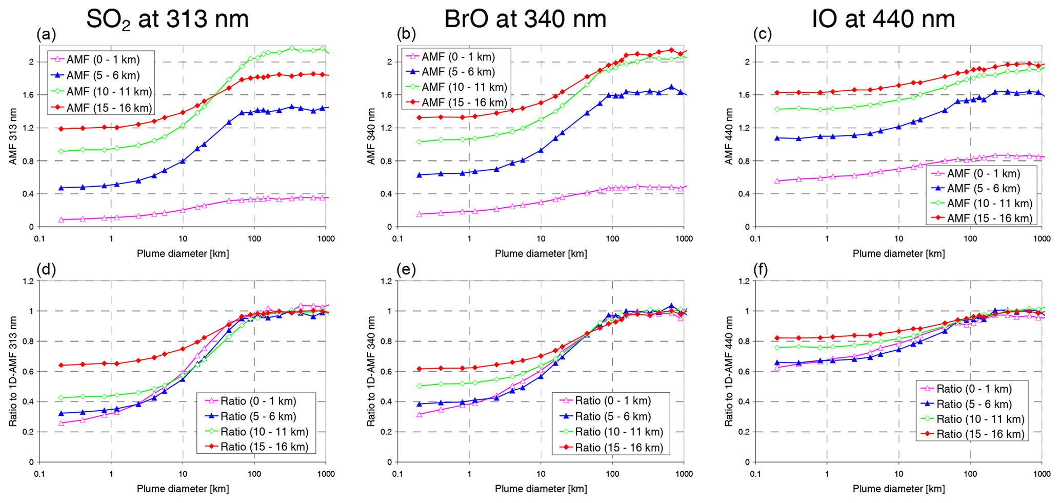
Figure 5 Dependence of the AMF on the horizontal plume extension. (a–c) AMFs for different plume altitudes and wavelengths; (d–f) AMFs normalised by the corresponding 1D AMFs (assuming a horizontally extended plume). The simulations are performed for SZA 0^∘, VZA 0^∘, FOV 0.014^∘, satellite altitude 824 km a.s.l. and no aerosols.

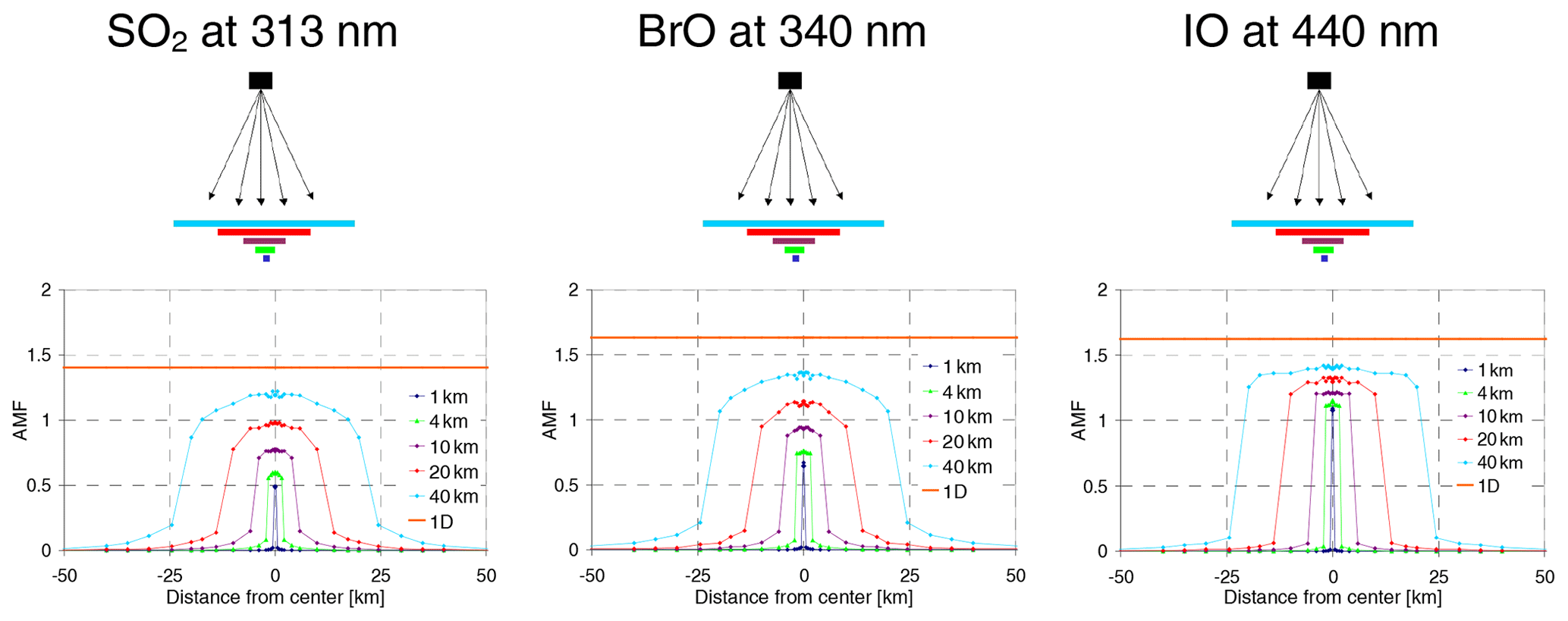
Figure 6 AMFs for plume scans in near-nadir viewing geometry (SZA = 0^∘, VZA = 0^∘) at different wavelengths. It is assumed that the satellite scans the plume with a narrow FOV (∼ 0.014^∘). The different colours represent AMFs for plumes at 5–6 km altitude and with different horizontal extensions (from 1 × 1 km² to 40 × 40 km²). Results for other plume altitudes are shown in Appendix C.

In Fig. 6, so-called plume scans for plumes with different horizontal extensions are presented for a plume altitude of 5–6 km (results for other plume altitudes are shown in Fig. C1 of Appendix C). The highest AMFs occur directly above the plume centre, but even these AMFs are systematically smaller compared to the corresponding 1D AMFs (orange horizontal lines). The deviation is strongest for short wavelengths and narrow plumes. The AMFs slightly decrease from the plume centre towards the edges. Outside the plume they decrease rapidly but stay clearly above zero.

This “smoothing” of the AMF (compared to the horizontal extent of the plume) reflects the effect of horizontal photon paths and is directly connected to the atmospheric visibility. Towards short wavelengths, the free photon paths become shorter and the scattering probability becomes higher. Thus, the smoothing effect is strongest at short wavelengths. These general dependencies are also found for other plume altitudes (see Fig. C1 in Appendix C), but the absolute values of the AMFs strongly increase with increasing plume height for both narrow plumes and horizontally extended plumes (while the ratios of the AMFs for narrow plumes to those of horizontally extended plumes are similar for the different plume altitudes).

One interesting question is whether the decrease in the AMF above the plume (compared to the 1D AMF) and the increase outside the plume (compared to a AMF of zero) exactly compensate each other. Indications of such a compensation are illustrated in Fig. 7 (note that, for a quantitative interpretation, two horizontal dimensions have to be considered). To answer this question, simulations for satellite observations with a very large FOV corresponding to a ground pixel size of 200 × 200 km² are performed. Such large ground pixels are larger than typical horizontal photon paths (see Table 2). Thus, almost all photons which have “seen” the trace gas plume will stay inside the FOV.

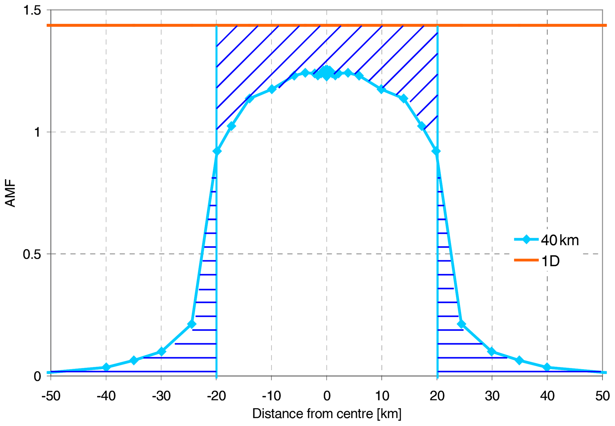
Figure 7 AMFs for plume scans (as in Fig. 6) in near-nadir viewing geometry (SZA = 0^∘) for SO₂ (weak) at 313 nm and a plume at 5–6 km altitude. In the area of the plume the AMFs are smaller than the 1D AMF, whereas outside they are larger than zero. The differences are indicated by the blue-marked areas for a plume of 40 × 40 km².

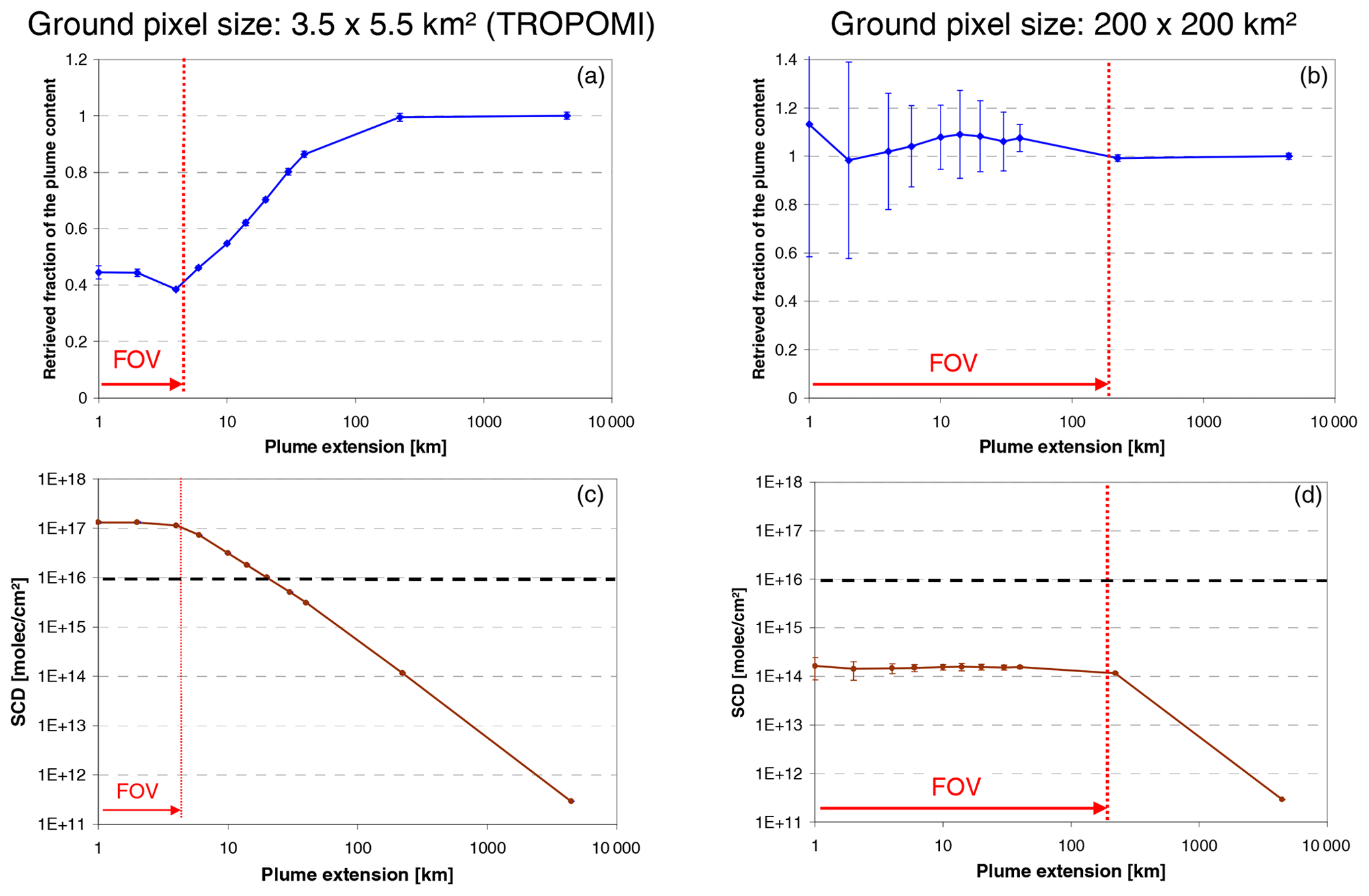
Figure 8 (a, b) Retrieved fraction of the plume content as a function of the horizontal plume extension (note the logarithmic scale) for measurements of SO₂ at 313 nm. (c, d) Measured SO₂ for a SO₂ VCD (for a 1 × 1 km² pixel) of 1 × 10¹⁸ molec cm⁻². The horizontal dashed line indicates the detection limit (assuming an OD threshold of 0.001). (a, c) Results for a TROPOMI ground pixel; (b, d) results for a large ground pixel of 200 × 200 km². Note that in the case of plume size greater than ground pixel size, only the fraction of the plume within the ground pixel size is considered. Simulations are for a plume altitude from 5 to 6 km, a wavelength of 313 nm, VZA = 0 and SZA = 0^∘. The error bars represent the standard deviation calculated from 40 individual simulations. Results for other plume altitudes and molecules (wavelengths) are shown in Appendix C.

The simulation results (together with similar results for a TROPOMI FOV) for a wavelength of 313 nm and a plume height of 5–6 km are shown in Fig. 8 (results for other combinations of wavelengths and plume altitudes are shown in Fig. C2 in Appendix C). Panels a and b present the retrieved fraction of the plume content as a function of the horizontal plume extension. This fraction is defined as the ratio of the retrieved number of trace gas molecules using a 1D AMF and the true number of trace gas molecules of the plume (used as input in the radiative transfer simulations). The retrieved fraction of the plume content is calculated as follows. First the simulated SCD for 3D plumes is divided by the corresponding 1D AMF yielding the average VCD across the satellite ground pixel. This VCD is then multiplied by the area of the ground pixel size yielding the total number of molecules. Finally, this value is divided by the number of trace gas molecules used as input for the simulations. Note that if the satellite ground pixel is smaller than the plume, only the input number of plume molecules covered by the satellite ground pixels is used to calculate the retrieved fraction of the plume content.

For TROPOMI, the retrieved fractions of the plume amount largely underestimate (between about 15 % and 60 %, depending on altitude and wavelength) the input trace gas amounts for small plume sizes, in agreement with the results shown in Figs. 5 and 6. The largest underestimation occurs for short wavelengths and a plume size similar to the ground pixel size. This can be understood by the results of the plume scans shown in Fig. 6, where the AMFs at the plume edges are the smallest within the plume. For plumes larger than the TROPOMI ground pixel, the retrieved fraction of the plume content (within the ground pixel size) then increases with plume size, because these scenarios converge to the 1D scenario (horizontally homogeneous trace gas layer).

Interestingly, for the large FOV (corresponding to a satellite ground pixel of 200 × 200 km²), the retrieved fractions of the plume amount are close to unity independent of the plume size. This confirms the above expectation that the decrease in the AMF in the area of the plume (compared to the 1D AMF) and the increase in the AMF outside the plume (compared to zero) compensate each other. In conclusion, we find that the correct plume amount can be retrieved using 1D AMFs only for two extreme cases.

• a.

  The ground pixel size is much larger than the free photon path length and the plume size (Fig. 8b and d). However, in such cases the trace gas absorption is very weak and usually below the detection limit (see Fig. 8, bottom right). Thus, small/medium volcanic plumes can usually not be detected by instruments with a large ground pixel size.

• b.

  The plume is homogenous and much larger than the free photon path length (and the ground pixel size). While the first condition is usually not well fulfilled, the second condition is typically fulfilled for strong eruptions. However, such plumes are large and can usually be detected by satellite instruments with low spatial resolution (no observations with high spatial resolution are needed). For such large ground pixel sizes, the effect of horizontal gradients will also be rather small.

Thus, small plumes (like for small/medium volcanic eruptions or degassing events) can only be observed by sensors with a small ground pixel size (like TROPOMI). However, for such observations the retrieved trace gas amount will be systematically and strongly underestimated if 1D AMFs are applied in the data analysis.

3.2 Quantitative analysis for different ground pixel sizes taking into account the detection limit of the spectral retrieval

As shown in the previous section, all molecules of a volcanic plume could in principle be retrieved with a 1D AMF if the satellite ground pixel is large (greater than about 100 × 100 km²). Thus, even for satellite measurements with small ground pixels it should be possible to retrieve all molecules of a volcanic plume if the results of many neighbouring ground pixels (surrounding the volcanic plume) are summed up. However, since the AMFs for pixels outside the volcanic plume are typically rather small (Fig. 6), for most of the observations of neighbouring ground pixels the trace gas absorption will be below the detection limit. This finding is confirmed in Fig. 9, which shows simulation results for the trace gas scenarios for the weak absorbers introduced in Sect. 2.1. Here again it should be noted that these results are valid only for the assumed trace gas scenarios and detection limits. For higher plume amounts and/or lower detection limits, lower SCDs, e.g. those for the neighbouring pixels, might be above the detection limit. Moreover, for scenarios with constant emissions (degassing) and stable wind fields, several measurements could be averaged, which would also lower the detection limit which is usually determined by photon noise. Nevertheless, from these simulations we derive the following general conclusions.

• a.

  The trace gas SCDs from neighbouring pixels are usually rather small. For TROPOMI observations the ratios of the maximum SCDs from the neighbouring pixels relative to the SCDs of the centre pixel range from 2 % for 440 nm to 7 % for 313 nm. Thus, these measurements will often be below the detection limit.

• b.

  Even if measurements of the neighbouring pixels are above the detection limit, their contribution to the detected total plume amount is small. For the two closest neighbouring pixels (because of symmetry in total four), their additional contribution ranges from about 4 % (440 nm) to about 11 % (313 nm) (relative contributions with respect to the true plume content).

• c.

  For OMI, the SCanning Imaging Absorption spectroMeter for Atmospheric CHartographY (SCIAMACHY) or GOME-2, the SCDs of the neighbouring pixels are always below the detection limit for the scenarios (with narrow volcanic plumes) considered in Table 3.

Figure 10 shows the retrieved fraction of the plume molecules (for a 1 × 1 × 1 km³ plume at different altitudes) as a function of the ground pixel size for the three selected wavelengths. As discussed before, the strongest underestimation is found for TROPOMI and for short wavelengths. For SCIAMACHY and GOME-2 observations, the underestimation is only between a few percent and 15 %. However, for these sensors, the retrieved trace gas SCDs are below the detection limit for the narrow plumes considered here. Interestingly, very similar results are found for 313 and 340 nm, probably because of some compensating effects of the increase in the light-mixing effect but also an increase in the probability of multiple scattering towards shorter wavelengths. For plumes close to the surface (0–1 km altitude), very similar fractions are found to those for the plume between 5 and 6 km, but because of the decreasing sensitivity of the satellite observations towards the ground, the corresponding trace gas absorptions are smaller and, for the weak SO₂ scenario, even below the detection limit. For plumes at higher altitudes, the underestimation becomes smaller because the probability of multiple scattering due to Rayleigh scattering decreases and thus the differences in the AMFs for narrow and horizontally extended plumes become smaller.

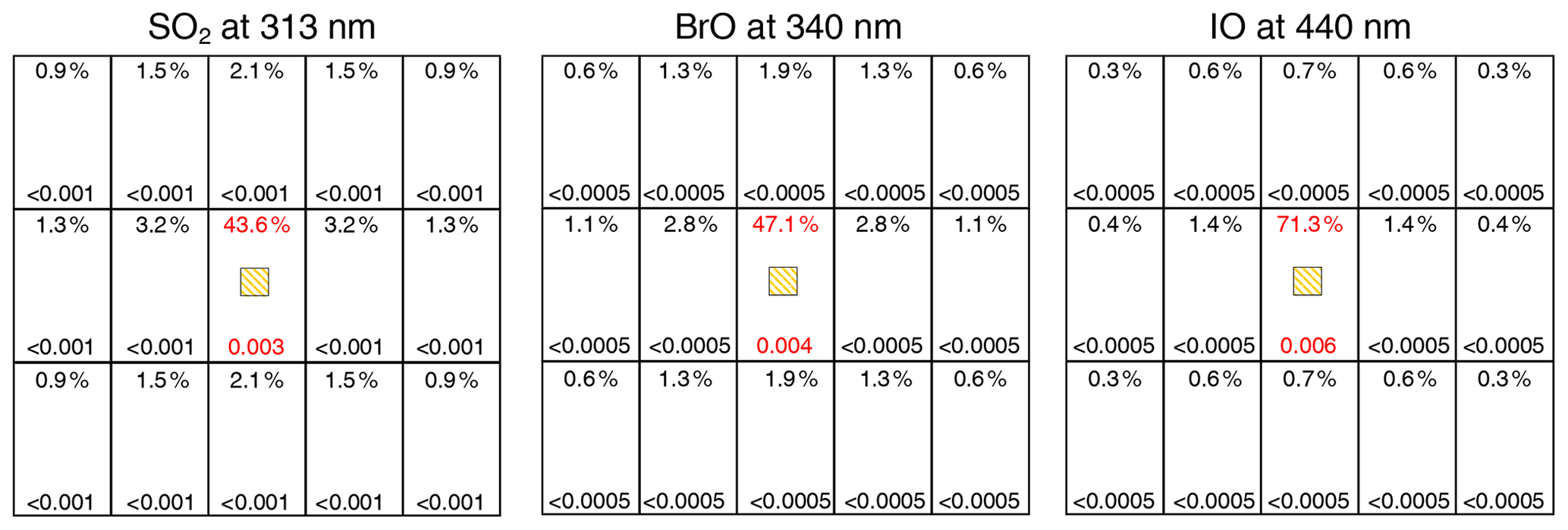
Figure 9 Horizontal coverage of a 1 × 1 × 1 km³ plume (yellow hatched areas) by TROPOMI observations at different wavelengths. The numbers at the tops of the TROPOMI pixels indicate the fractions of the plume molecules retrieved from that ground pixel. The numbers at the bottom indicate the optical depth of the trace gas absorption. Red values represent results above the respective detection limit.

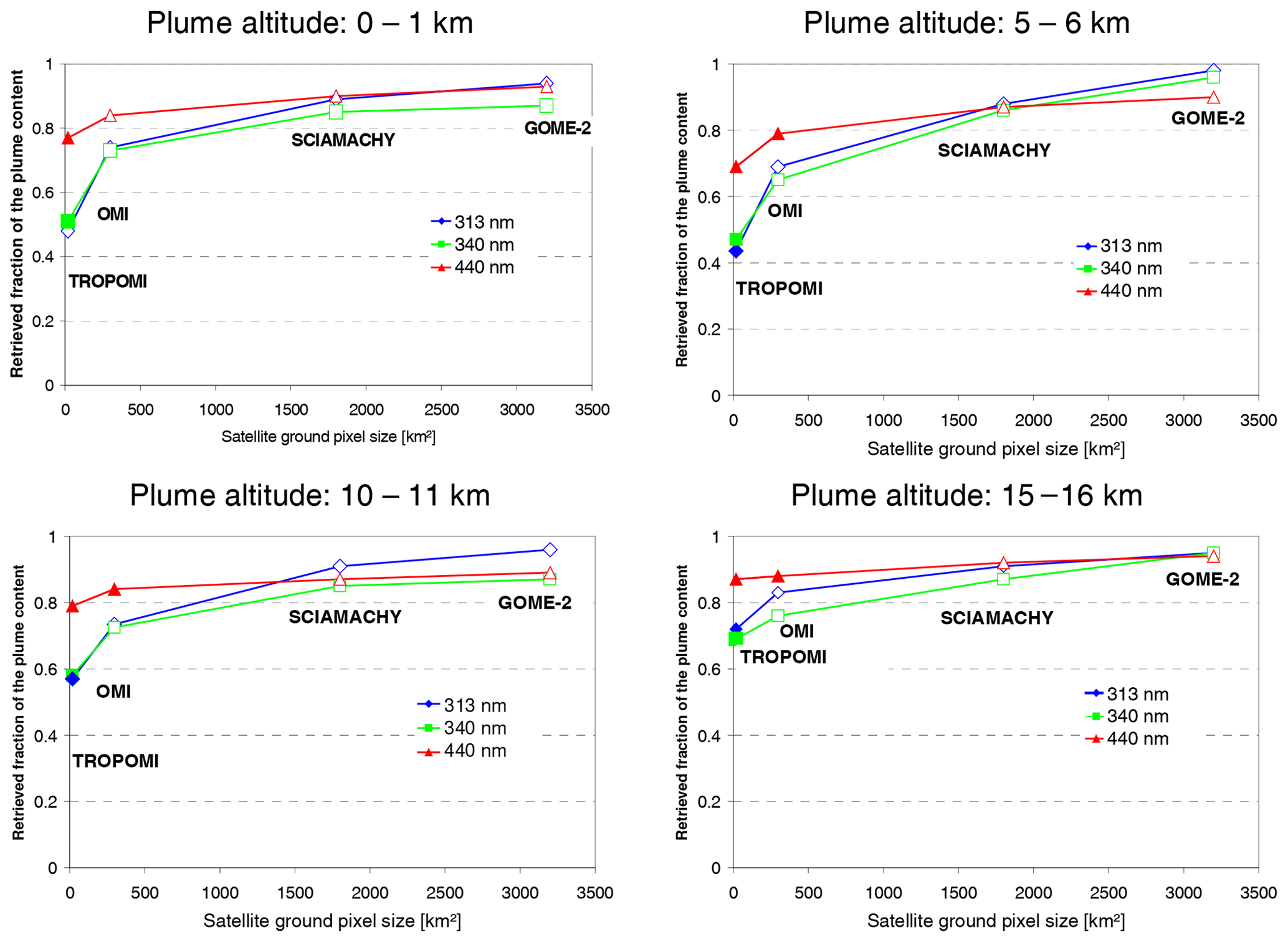
Figure 10 Retrieved fraction of the plume content for different satellite sensors (for a 1 × 1 × 1 km³ plume at different altitudes). Full symbols indicate observations above the detection limit. For the relatively large ground pixel sizes of SCIAMACHY and GOME-2, the errors are between 5 % and 10 %.

3.3 Influence of aerosols

Figure 11 presents AMFs (similarly to Fig. 6) and normalised radiances (radiance/irradiance) for plume scans in near-nadir viewing geometry (solar zenith angle, SZA = 0^∘) for different wavelengths (for SO₂ at 313 nm, BrO at 340 nm, and IO at 440 nm) and aerosol scenarios. The plumes are located between 5 and 6 km and contain the trace gas together with the aerosols (results for other plume heights are shown in Fig. C3 in Appendix C). Again, the amount of molecules in the plume is assumed to be constant (and homogenously distributed), and thus the trace gas VCDs and AOD vary with the horizontal plume extent (see Table 3). The aerosols are assumed to be either purely scattering (SSA = 1) or strongly absorbing (SSA = 0.8). The different colours in Figs. 11 and C3 represent AMFs and normalised radiances for plumes with different horizontal extensions (from 1 × 1 to 40 × 40 km²).

Figure 11 AMFs and normalised radiances for plume scans in near-nadir viewing geometry (SZA = 0^∘) for different wavelengths and aerosol contents. The satellite scans the plume with a narrow FOV (∼ 0.014^∘). The different colours represent AMFs for plumes at 5–6 km altitude and with different horizontal extensions (from 1 × 1 to 40 × 40 km²). The rather low radiance at 313 nm (in spite of the high probability of Rayleigh scattering) is caused by the stratospheric ozone absorption. Results for other plume altitudes are shown in Appendix C.

For small plume extensions (and thus high AOD in the plume), a strong effect of aerosols is seen (except for short wavelengths and plumes close to the surface): for the scenarios with scattering aerosols, both the AMF and the normalised radiance increase compared to the scenarios without aerosols (Fig. 6). For the scenarios with absorbing aerosols, the opposite is found. For the interpretation of the simulated radiances, it is important to take into account that, especially for the low-altitude plumes, a substantial fraction of the atmospheric molecules is still located above the volcanic plume, which scatters the sunlight towards the instruments without having seen the plume. Thus, even for narrow plumes with absorbing aerosols, the reduction in the observed radiance above the plume is relatively small. The low radiances at 313 nm are caused by the stratospheric ozone absorption, which is negligible at longer wavelengths.

For observations with an extended FOV, the effective AMF results from the spatial averaging of the AMF weighted by the radiance. In that way the increased (decreased) radiance above scattering (absorbing) aerosols further increases (decreases) the AMFs for scattering (absorbing) aerosols. As a consequence, aerosols can have a rather strong impact on the effective AMF compared to the scenarios without aerosols.

In Fig. 12 the retrieved ratios of the plume content (ratio of the retrieved number of trace gas molecules assuming a 1D AMF and the true number of trace gas molecules in the plume) for TROPOMI observations are shown for aerosol scenarios (for a 1 × 1 × 1 km³ plume). Compared to the results for the aerosol-free cases, the results are higher (for scattering aerosols) or lower (for absorbing aerosols). The strongest differences are found for IO at 440 nm, because the relative effect of the aerosols compared to Rayleigh scattering increases towards longer wavelengths. For scattering aerosols, the true plume content can even be overestimated due to the light path enhancement from increased multiple scattering in the plume and more back-scattered light from the plume (higher reflectance above the plume). Very similarly to the scenarios without aerosols, the ratios of the maximum SCDs of the neighbouring pixels to the SCDs of the centre pixels range from 2 % to 9 %.

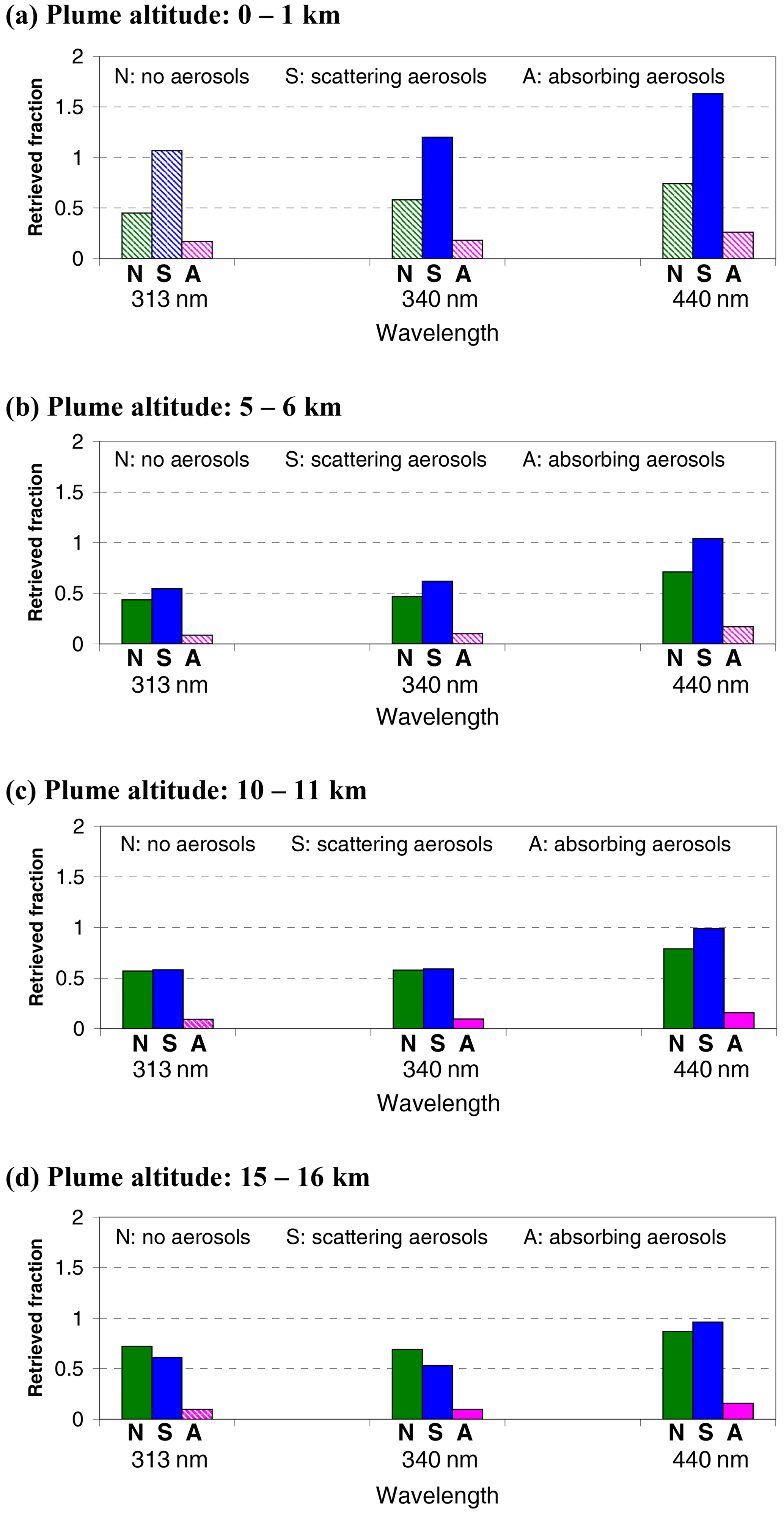
Figure 12 Retrieved fraction of the plume content at different wavelengths for different plume heights and aerosol scenarios for TROPOMI observations (horizontal plume extension 1 × 1 km²). Hatched bars indicate scenarios for which the absorption is below the detection limit for the weak trace gas scenarios described in Sect. 2.1 (results for the satellite pixel directly above the plume).

4 Saturation effect

For strong atmospheric absorbers like SO₂, the exact plume extent becomes especially important. If the same amount of molecules is confined in a small or large volume (depending on the dilution state of the plume), the corresponding VCDs and vertical optical depths vary. For narrow horizontal plume extensions (e.g. in fresh plumes before effective mixing with ambient air), the optical depth is higher than for more diluted plumes (Fig. 2b). This effect is illustrated in Fig. 13 for SO₂ observations at a wavelength of 313 nm (representative of the standard SO₂ fit range; see Fig. 4) and a plume height of 5–6 km. Results for other plume heights are shown in Fig. C4 in Appendix C. In the left part of the figure the spatial distributions of the SO₂ VCDs are shown for the scenarios with SO₂ as a weak absorber (top), “strong,1” (middle) and “strong,4” (bottom); see Table 3. The different colours indicate the different horizontal extensions of the plume (with the total amount of molecules kept constant). In the centre and right parts of the figure, plume scans of the AMF and the back-scattered normalised radiance are shown. As expected, for the scenario with SO₂ as a weak absorber, even for the smallest horizontal plume extension (1 × 1 km²), the radiance above the plume is the same as outside the plume (top right). The decrease in the AMF compared to the 1D AMF is thus simply a result of the light-mixing effect (Sect. 3). For higher SO₂ concentrations, however (middle and bottom panels), the radiance is systematically reduced above the plume (like for the scenario with strong aerosol absorption; see Fig. 11, bottom), because a substantial fraction of the photons is absorbed by SO₂. Here it is interesting to note that even for the highest SO₂ concentrations the radiance does not approach zero, indicating that part of the light is back-scattered from molecules above the volcanic plume (while almost all photons reaching the volcanic plume are probably absorbed by SO₂). Accordingly, with increasing plume height a stronger reduction in the observed radiance for plumes with high SO₂ amounts is found (see Fig. C4 in Appendix C). For the scenarios with high SO₂ amounts, the AMFs above the plume are also systematically reduced compared to the scenarios with weak SO₂ absorption, because the SO₂ absorption is so strong that the observed photons have only seen part of the vertical plume extension (similar to the scenario with strong aerosol absorption; see Fig. 11, bottom). The combined effects of reduced back-scattered radiance and reduced AMFs strongly reduce the effective AMFs when averaged over a satellite ground pixel. The reduction in the AMF is largest for the narrow plumes.

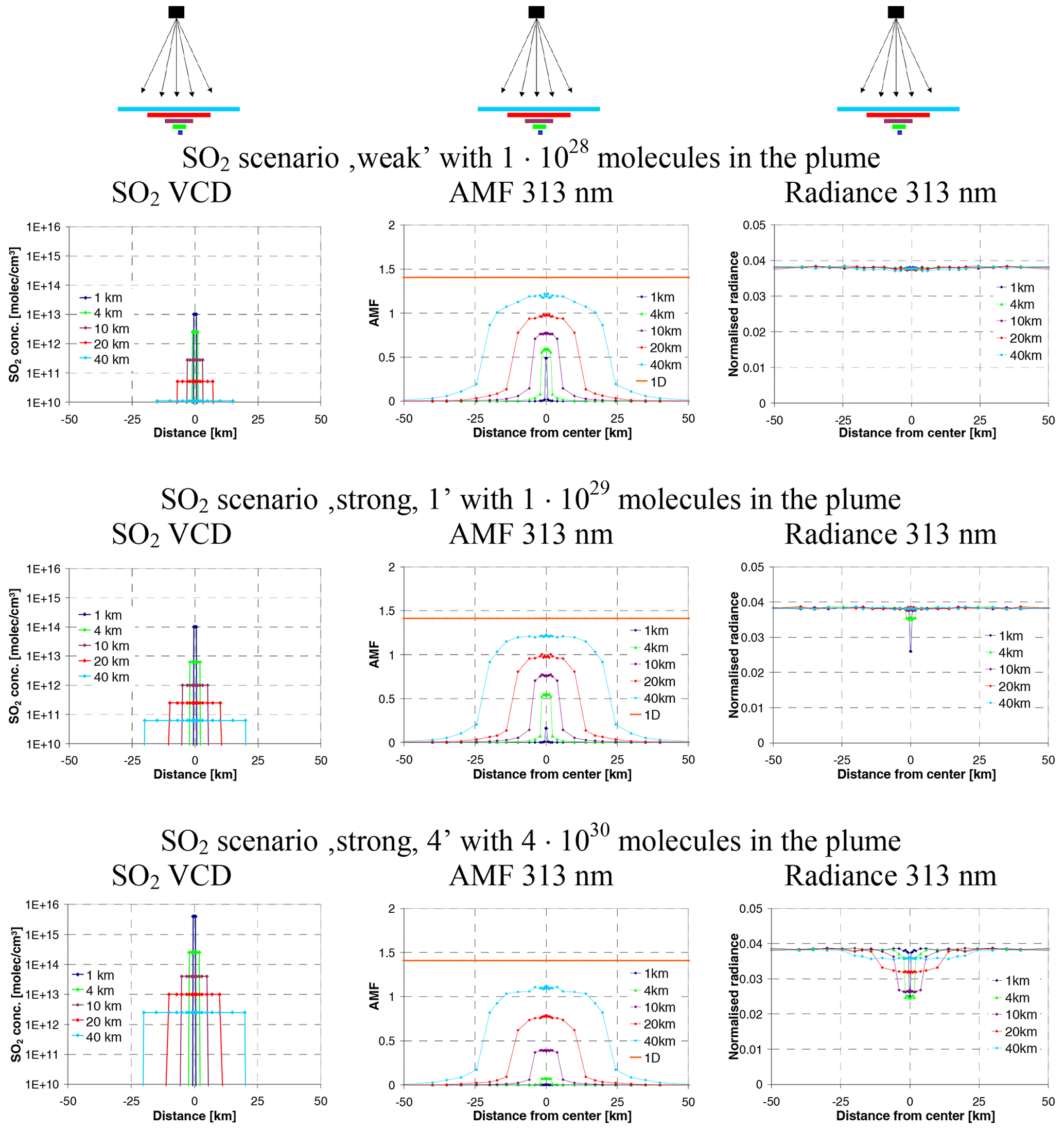
Figure 13 Plume scans for SO₂ plumes with different amounts of molecules and different horizontal extensions (for the different SO₂ scenarios, see Table 3). Left: SO₂ VCDs of the plumes; middle: AMFs at 313 nm; right: normalised radiances at 313 nm. Here only the scenarios “weak”, “strong,1” and “strong,4” are considered to illustrate the transition from cases with no saturation to cases with medium or strong saturation. The additional intermediate scenarios “strong,2” and “strong,3” are later also used for the quantification of the saturation effect for the different plume extensions (Fig. 14) and satellite instruments (Fig. 15). Results for other plume altitudes are shown in Fig. C4 in Appendix C.

4.1 SO₂ results for TROPOMI observations for different plume contents and wavelengths

Figure 14 shows the fraction of the retrieved plume content for a plume at 5–6 km altitude as a function of the plume size derived from TROPOMI observations if a 1D AMF is assumed in the analysis. In addition, the retrieved SO₂ SCDs are shown. Similar results for other plume altitudes are shown in Fig. C5 in Appendix C. The simulations are performed for the four scenarios with strong SO₂ absorption (see Table 3) and four wavelengths (313.1, 324.15, 332.0, 370.3 nm; see Table 4 and Fig. 4). From the results in Figs. 14 and C5, several conclusions can be drawn.

• a.

  A systematic and strong underestimation for short wavelengths is found (in addition to the light-mixing effect). This additional underestimation is caused by the strong SO₂ absorption for narrow plumes and is referred to in this study as the saturation effect. The underestimation caused by the saturation effect is similar for the different plume heights.

• b.

  In spite of the strong SO₂ absorption, in some cases, the retrieved SO₂ SCDs are below the threshold value (red horizontal line), above which the operational SO₂ retrieval switches to the alternative fit windows (at longer wavelengths). The threshold values are 4 × 10¹⁷ molec cm⁻² for the switch from fit range 1 to fit range 2 and 6.7 × 10¹⁸ molec cm⁻² for the switch from fit range 2 to fit range 3; see Theys et al. (2021b). This is an important finding, because in such cases no analyses in the alternative fit windows will be performed, and such high SO₂ amounts stay undetected in the current TROPOMI SO₂ retrieval. In contrast to the underestimation caused by the saturation effect, the retrieved trace gas SCDs depend strongly on the plume altitude.

• c.

  To retrieve the correct SO₂ SCD (and to avoid the saturation effect), it is recommended that simultaneous analyses in different wavelength ranges are performed. If the SCDs at shorter wavelengths are found to be systematically smaller than those at longer wavelengths, the results of the retrievals at the longer wavelengths should be considered. Only if in the standard fit window similar SCDs are obtained as at longer wavelengths should the results from the standard fit window be used. This procedure would prevent high SO₂ amounts from staying undetected. Specific thresholds for the differences in the results in the different fit windows should be defined in a dedicated and more detailed study, also taking into account the increasing detection limits towards longer wavelengths.

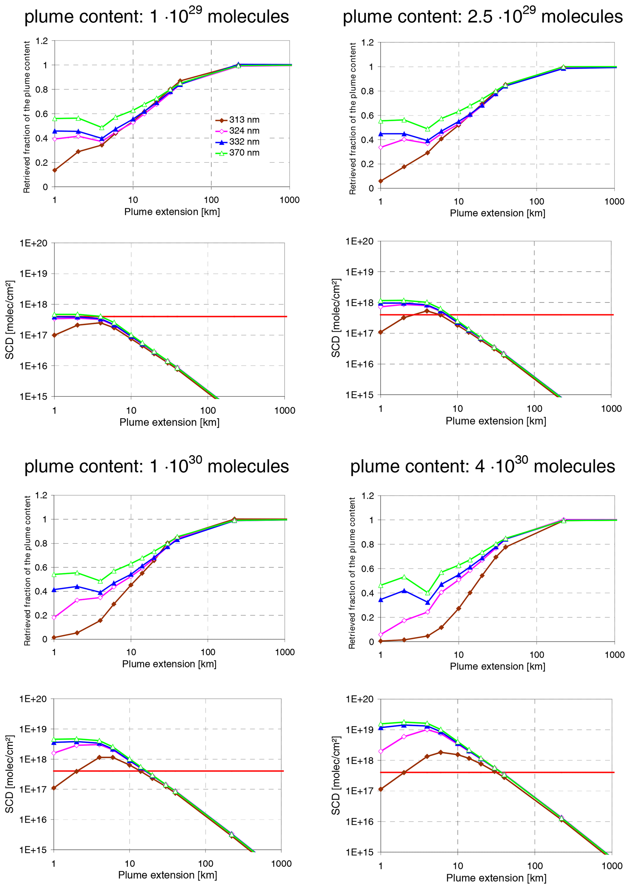
Figure 14 Retrieved fraction of the plume content (top) and SO₂ SCDs (bottom) from TROPOMI measurements at different wavelengths as a function of the plume size and for different amounts of molecules in the plume (plume height: 5–6 km). The red horizontal line indicates the threshold, above which the operational SO₂ retrieval switches from the standard fit window to the first alternative fit window (at longer wavelengths). Results for other plume altitudes are shown in Appendix C.

4.2 SO₂ results for observations from different satellites

Figure 15 presents an overview of the fraction of the retrieved SO₂ content of the plume by different satellite instruments for scenarios with strong absorptions (see Table 3) for a 1 × 1 × 1 km³ plume at 5–6 km altitude. Similar results for other plume altitudes are shown in Fig. C6 in Appendix C. For all SO₂ scenarios a strong dependence of the retrieved SO₂ SCD (and the retrieved fraction of the plume content) is found. The wavelength above which the underestimation becomes negligible depends on the SO₂ scenario (see Table 3). For high SO₂ amounts, only analyses at long wavelengths yield reasonable results (but are of course still affected by the light-mixing effect). Interestingly, the saturation effect is similar for the different instruments (with different ground pixel sizes), indicating that the saturation effect is mainly determined by the plume properties. Overall, similar results for the different plume heights are found, but for plumes at high altitudes a difference is found for the longer wavelengths compared to plumes at lower altitudes: there the retrieved fraction of the plume content increases, especially for the instruments with small pixel sizes (TROPOMI and OMI), because the light-mixing effect becomes less efficient with increasing altitude due to the reduced probability of multiple Rayleigh scattering.

Figure 15 Retrieved fractions of the plume content and SO₂ SCDs for different satellite instruments and for a plume size of 1 × 1 km² as a function of the wavelength (plume altitude 5–6 km). The full symbols represent measurements with SCDs above the detection limit. Note that for the rather large ground pixel sizes of SCIAMACHY and GOME-2 the errors are between 5 % and 10 %. Results for other plume altitudes are shown in Appendix C.

4.3 Effect of the wavelength dependence of the AMF

So far the simulations were performed at single wavelengths in order to save computation time. These wavelengths were chosen to represent the dominant differential absorption cross sections for the different SO₂ fit windows (see Fig. 4 and Table B1). While these monochromatic simulations can give a good first indication of the saturation effect, they neglect the effect of the wavelength dependence of the AMF (Marquard et al., 2000; Puķīte et al., 2010; Puķīte and Wagner, 2016). This wavelength dependence is mainly caused by the wavelength dependence of the SO₂ absorption cross section, because for increasing absorption cross sections the penetration depth of the back-scattered photons (and hence the AMF) decreases: the AMF is smallest for the highest values of the cross sections, and the wavelength dependence of the AMF leads to a further decrease in the differential optical depth:

$$\begin{array}{}\text{(2)}& \mathit{\tau }\left(\mathit{\lambda }\right)=\mathrm{VCD}\cdot \mathrm{AMF}\left(\mathit{\lambda },\mathit{\sigma }\left(\mathit{\lambda }\right)\right)\cdot \mathit{\sigma }\left(\mathit{\lambda }\right).\end{array}$$

Note that an additional wavelength dependency of the AMF due to Rayleigh scattering is less important for the rather small fit windows considered here. We quantify the effect of the wavelength dependence of the AMF as described in Appendix D.

It is found that the effect of the wavelength dependence of the AMF is small for cases with small optical depths. For cases with high optical depths and thus strong saturation effects, the true underestimation becomes larger than for the monochromatic AMFs. However, such cases can be easily identified by the comparison of the retrieved SO₂ SCDs from different spectral ranges. For the SO₂ analysis, an appropriate spectral range (with a negligible saturation effect) then has to be selected. For such analyses, the effect of the wavelength dependence of the AMF also becomes negligible.

5 Geometric effects for elevated plumes

The simulations presented so far were carried out for scenarios with overhead Sun (SZA = 0) and nadir-viewing instruments (viewing zenith angle, VZA = 0). These scenarios were chosen to investigate the light-mixing and saturation effects in a fundamental way. In typical measurement situations, however, the illumination and viewing directions deviate from the vertical axes. Especially for elevated plumes, the trace gas absorption will then not be seen for the ground pixel exactly below the plume (Fig. 2c). In extreme cases, even double plumes might be observed. These effects of slant illumination and viewing angles are referred to as geometric effects in this study and are investigated in this section. Geometric effects lead to an increase in the horizontal extension over which the plume signal is seen compared to the observation geometry with SZA = VZA = 0. However, at the same time, the magnitude of the absorption also decreases and might effectively fall below the detection limit. This reduction in the absorption is simply caused by the fact that for such cases the atmospheric light paths cross the plume only once (or less) for a given viewing angle.

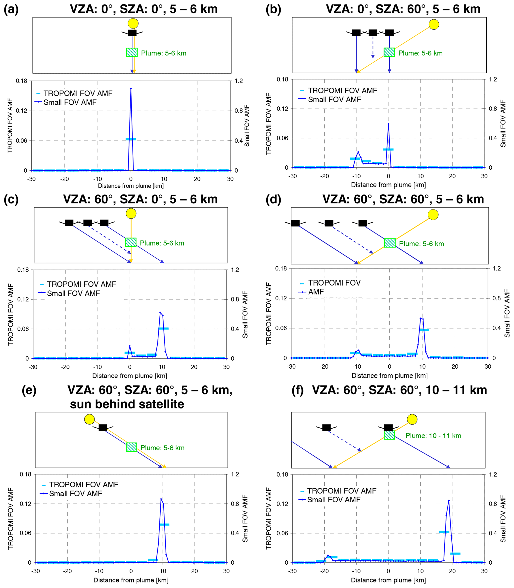
Figure 16 AMFs for TROPOMI observations of elevated plumes for different combinations of SZA and VZA. The blue lines show the AMFs for observations with a narrow FOV (∼ 0.014^∘) (right y axis). The bright-blue symbols represent simulations with a TROPOMI FOV (left axis). All simulations are for IO at 440 nm and plume sizes of 1 × 1 × 1 km³. Results for 313 nm (SO₂) and 340 nm (BrO) are shown in Figs. E1 and E2 in Appendix E.

In Fig. 16 the AMFs for plume scans for observations of elevated plumes with various combinations of SZA and VZA are shown. The blue lines show the AMFs for observations with a narrow FOV (right y axis); the bright-blue horizontal bars represent simulations for a TROPOMI FOV (3.5 km in the across-track dimension, left axis). Note that we kept the ground pixel size constant (3.5 × 5.5. km²) for all viewing angles in order to study the basic effects in a systematic way. For real TROPOMI observations, the ground pixel sizes increase for slant viewing angles. The TROPOMI AMFs are systematically lower than the AMFs for the narrow FOV, because the plume covers only a small fraction of the TROPOMI ground pixel (for nadir view ∼ 5 %).

Figure 17 Number of satellite pixels with SCDs above the detection limit (a, c, e) and the retrieved fraction of the plume content (b, d, f) for TROPOMI observations of SO₂ (weak, 313 nm), BrO (340 nm), and IO (440 nm) with different viewing and solar zenith angles. The plume has an extension of 1 × 1 × 1 km³ and is located at 5–6 km altitude. The red circles indicate scenarios with the Sun and the satellite in the same direction for which the smearing effect is smallest. RAA indicates the relative azimuth angle between the viewing direction and the Sun. Here a RAA of 180^∘ represents cases where the Sun shines in the same direction as the satellite view.

The simulations shown in Fig. 16 are performed for 440 nm (IO). Similar results but with less-clear peaks are obtained for the other wavelengths (for SO₂ at 313 nm and BrO at 340 nm; see Figs. E1 and E2 in Appendix E). In addition to the AMFs, sketches of the corresponding observation geometries are also shown above the sub-figures. As expected, the plume signals seen by the satellite are usually not found for those ground pixels covering the plume. Instead, maxima of the AMF are found for the downward and upward light paths crossing the plume, but slightly enhanced values are also found in between these maxima. They are caused by sunlight which has crossed the plume and is then scattered towards the instrument before it reaches the ground. As a general finding, the apparent horizontal extent of the plume increases for observations with slant illumination and/or slant viewing angles compared to observations with SZA = VZA = 0. At the same time the magnitude of the AMF decreases for observations with slant illumination and/or slant viewing angles. Both aspects have a direct influence on the retrieved fraction of the plume content: on the one hand, the “smearing” of the plume signal can lead to a larger number of ground pixels with enhanced absorptions and thus to a larger total covered area. On the other hand, ground pixels with weak absorptions (e.g. between the two AMF maxima) might fall below the detection limit (especially for scenarios with low trace gas VCDs). Both dependencies are seen in Fig. 17, where the number of pixels above the detection limit and the retrieved fraction of the plume content for TROPOMI observations with various viewing and illumination angles are shown for different scenarios of weak absorbers (see Table 3). For the different trace gases, different numbers of pixels with SCDs above the detection limit are found. The largest numbers are found for IO at 440 nm (weakest probability of Rayleigh scattering) and slant viewing and illumination angles (with opposite direction, relative azimuth angle RAA = 0^∘), for which the apparent spatial extent of the plume becomes largest. Interestingly, the retrieved fraction of the plume content is similar for all viewing geometries.

6 Plume side-effects for low plumes

For slant illumination and viewing angles, interactions of photons with the sides of the plumes can become important, especially for plumes containing aerosols. However, even for plumes free of aerosols, photons entering or leaving the plumes from the sides have seen different trace gas absorptions compared to the 1D scenarios. In this section plume side-effects are investigated for TROPOMI observations and for a narrow plume (1 × 1 × 1 km³) located directly above the surface. We chose this low plume altitude, because for such plumes the side-scattering effect can be investigated without interference with the geometric effects (Sect. 5). Of course, the side-scattering effect also affects plumes at higher altitudes (in addition to geometric effects). The aerosol scenarios are similar to those in Sect. 2.2, with an AOD of 10 and a single-scattering albedo of 1.0 (purely scattering aerosols) or 0.8 (strongly absorbing aerosols).

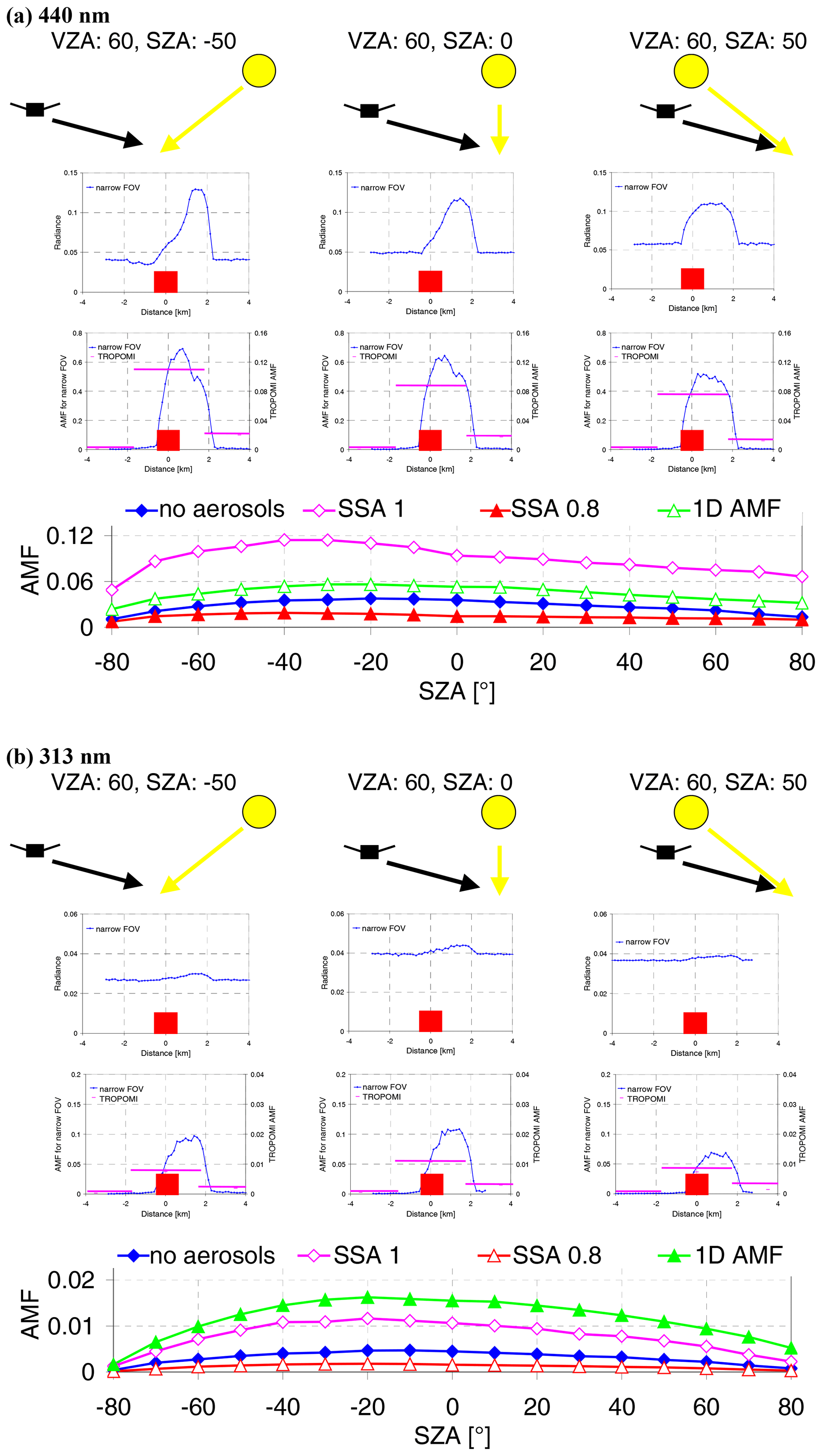
Figure 18 Dependence of the AMF and normalised radiance for a slant viewing angle (VZA = 60^∘) on the illumination angle for IO at 440 nm (a) and SO₂ at 313 nm (b). The upper panels show sketches of the investigated viewing and illumination angles (SZAs of −50, 0, and 50^∘). The middle panels show the normalised radiances and AMFs for these scenarios (for plumes with scattering aerosols) as a function of the relative distance from the plume (1 × 1 × 1 km³, red boxes). Note the different y axes for the AMFs calculated for a narrow FOV (left) or TROPOMI FOV (right). The plume is located directly above the surface (0–1 km). The bottom panels show the AMFs for a TROPOMI FOV as a function of the SZA (also for a VZA of 60^∘). The different lines represent 3D AMFs for plumes without aerosols (blue), with scattering (magenta) and absorbing (red) aerosols and the 1D AMF (without aerosols).

In the middle panels of Fig. 18a and b, the AMFs and normalised radiances for plume scans with a narrow FOV (0.014^∘) for (a) IO at 440 nm and (b) SO₂ at 313 nm are shown (blue symbols). The simulations are performed for a slant viewing angle (VZA = 60^∘) and selected SZAs (0 and 50^∘ in the forward and backward directions). The plumes of 1 × 1 × 1 km³ are located at the surface (red boxes) and contain the trace gas and scattering aerosols with an AOD of 10. In addition to the AMFs for the narrow FOV, AMFs for a TROPOMI FOV (3.5 km in the across-track direction) are also shown (horizontal magenta bars). For IO at 440 nm the normalised radiances and AMFs for the narrow FOV especially show complex dependencies on the viewing angle. Moreover, while the enhanced values of the radiances and the AMFs are found at similar viewing angles, there are also systematic differences in the details of their viewing angle dependencies. These are caused by the different sensitivities of both quantities on the atmospheric light paths. While the radiance mainly depends on the probability of scattering (on molecules and aerosols), the AMF also strongly depends on the length of the light path through the trace gas plume. These dependencies can be e.g. seen in the upper left part of Fig. 18a, where the maximum of the radiance is found at about 1.5 km, while the maximum AMF is found at a distance of about 0.8 km from the plume centre. Also, clear differences for forward and backward illumination are found. The stronger and more structured signals for IO at 440 nm are caused by the fact that the direct sunlight can penetrate deeper into the atmosphere than at shorter wavelengths, and thus geometric effects (like shadowing for a VZA of 60^∘ and a SZA of −50^∘) are more clearly visible. Also, the AMFs for the TROPOMI FOV differ systematically for different illumination directions. The TROPOMI AMFs (for ground pixels covering the plume) as a function of the SZA and for different aerosol scenarios) are shown in the bottom panels of Fig. 18 (also for a VZA of 60^∘). In addition to the 3D AMFs, the corresponding 1D AMFs (without aerosols) are also presented. A clear dependence on the SZA is found for all AMFs, which is slightly asymmetric (for forward and backward illumination) for the non-nadir viewing direction (VZA = 60^∘). These dependencies are caused by two effects: first the angular dependence of Rayleigh scattering which is relevant for both the 1D and 3D simulations, second the angular dependence of Rayleigh scattering and aerosol scattering (if aerosols are present) for the 3D plumes.

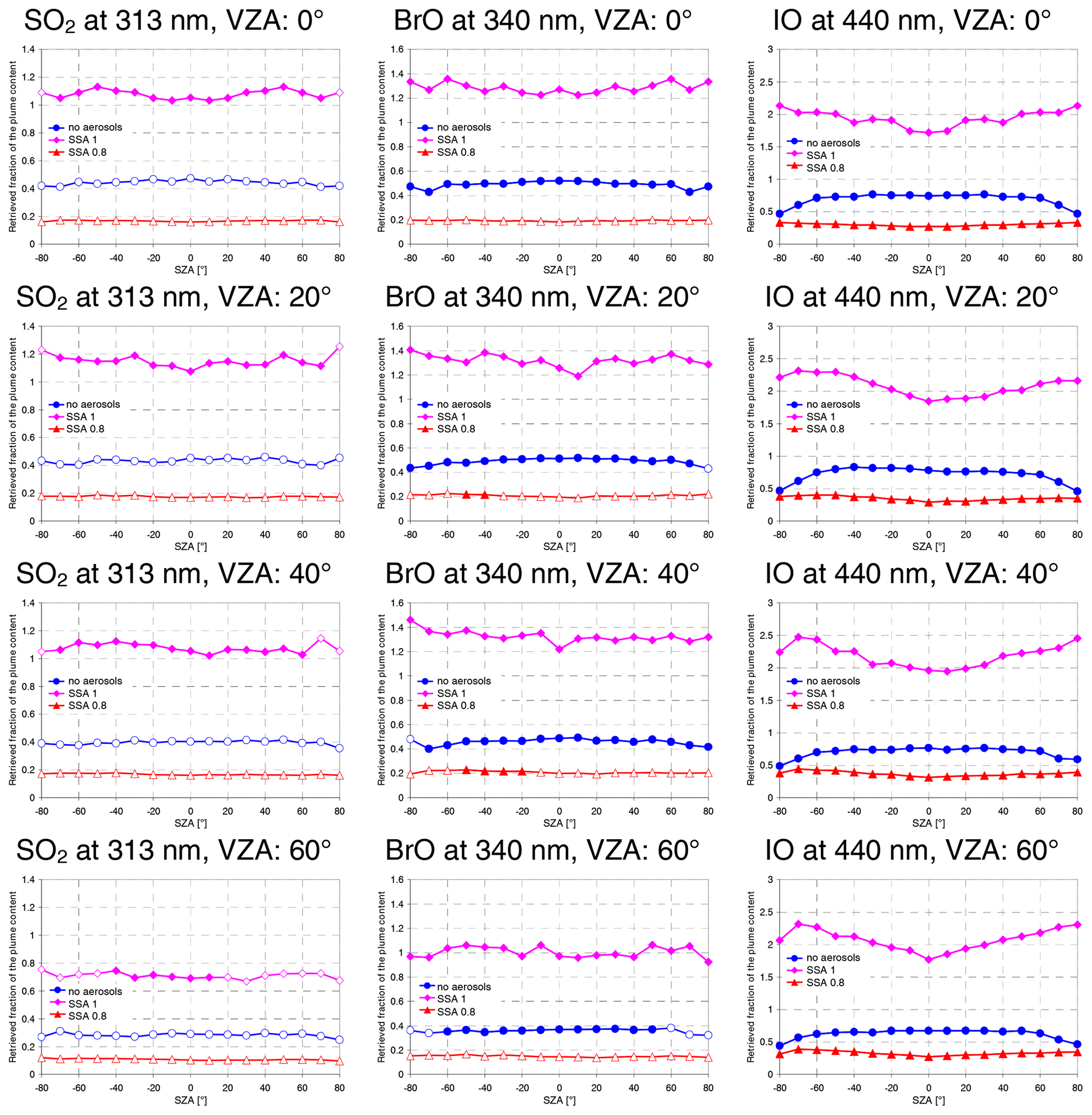
Figure 19 Retrieved fraction of the plume content for SO₂ (weak) at 313 nm (left), BrO at 340 nm (centre) and IO at 440 nm (right) as a function of the SZA for different viewing angles (blue: plume without aerosols; magenta: plume with scattering aerosols; red: plume with absorbing aerosols). Symbols in full colour represent results above the detection limit.

Figure 19 shows the retrieved fraction of the plume content for the different 3D cases if the corresponding 1D AMF is applied in the data analysis (similar to Fig. 12). For SO₂ at 313 nm and BrO at 340 nm, only weak dependencies on the SZA are found, indicating that at these short wavelengths the direct sunlight does not penetrate deeply into the atmosphere (because of the high probability of Rayleigh scattering). Also, only a weak dependence on the viewing angle is found. The low AMFs for the VZA of 60^∘ are related to the fact that for such slant angles the FOV for a 3.5 km-wide ground pixel is rather small, and not the whole vertical extent of the 1 × 1 × 1 km³ plume falls within the FOV.

In contrast to 313 and 340 nm, for IO at 440 nm systematic dependencies of the retrieved fraction of the plume content on the SZA are found, indicating the increased penetration depth of the direct sunlight. For plumes without aerosols, almost constant values are found for SZA < 70^∘, while for SZA ≥ 70^∘ the values strongly decrease. For observations of 3D plumes under such slant illumination angles, part of the direct sunlight does not cross the plume (like for the 1D scenario) before it is reflected/scattered towards the instrument. For the scenario with scattering aerosols, the retrieved fraction of the plume content is always > 1, indicating the effect of multiple scattering (together with the increased radiance from the plume providing more weight for the trace gas signal from the plume). The values systematically increase with an increasing SZA (except for the highest SZA). This increase is related to the higher contribution of photons entering the plume from the sides (pronounced forward scattering). For the non-nadir observations (VZA ≠ 0), a slight asymmetric dependence on the SZA is also found.

For the scenario with absorbing aerosols, low values and almost no SZA dependence are found for all wavelengths, indicating that the aerosol absorption prevents the penetration of the solar photons deep into the volcanic plume (together with the reduced radiance from the plume). In summary, as already shown in Sect. 3.3, the 3D AMFs (and thus the retrieved fraction of the plume content) for plumes with scattering aerosols can be strongly increased compared to aerosol-free plumes. This overestimation is strongest for long wavelengths. In such cases the satellite measurements strongly overestimate the true plume content if a 1D AMF is applied up to > 100 % towards a high SZA and a high VZA (note that the largest VZAs for such observations are about 66^∘, as e.g. for TROPOMI). Interestingly, the retrieved fraction of the plume content at 313 nm is close to unity regardless of the geometry.

For observations of plumes without aerosols or with absorbing aerosols, the satellite measurements strongly underestimate the number of plume molecules if a 1D AMF (without aerosols) is applied in the data analysis (in agreement with the results shown in Sect. 3.3).

7 Ground-based measurements

Three-dimensional effects are not only important for satellite observations of volcanic plumes, but also for ground-based observations. In this section we briefly deal with this topic but only discuss the light-mixing effect for ground-based observations, because it is the most fundamental 3D radiative transfer effect. Kern et al. (2010) investigated 3D effects for ground-based observations of volcanic plumes. Their focus was on the effect of sunlight scattered into the line of sight of the instrument without having crossed the volcanic plume before, referred to as the light-dilution effect (see also Millán, 1980). The light-dilution effect is usually the dominant effect for such observations. While the exchange of light between the plume and outside the plume by multiple scattered photons was also included in their simulations, its contribution to the 3D radiative effects was not explicitly discussed.

In our simulations for ground-based observations, we therefore consider two scenarios (see Fig. 20).

• a.

  Ground-based observations for zenith direction and very small SZA (here 0.3^∘): in this scenario the single-scattered light must have crossed the narrow plume before it is scattered into the instrument (like for the satellite observations with SZA = VZA = 0; see Sect. 3). Thus, no direct sunlight is scattered into the line of sight of the instrument without having crossed the plume before. These results can be directly compared to the results for satellite observations.

• b.

  Ground-based observations for zenith direction and slightly larger SZA (here 10^∘): in this scenario the single-scattered light has not crossed the narrow plume before it is scattered into the instrument (like for scenarios in Kern et al., 2010).

Note that for both scenarios single-scattered light can also be scattered above the plume into the line of sight of the instrument, but these light paths do not fall under the definition of the light-dilution effect.

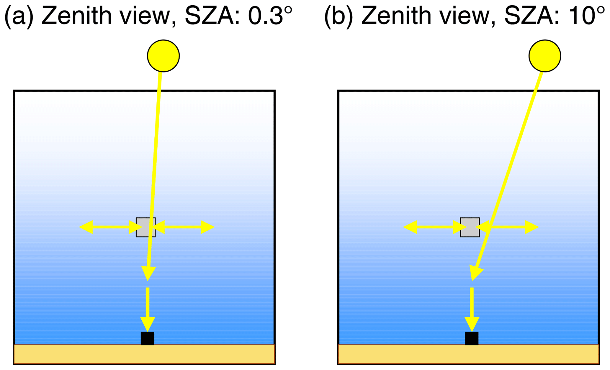
Figure 20 Ground-based observations of a narrow plume in the zenith direction. For an almost overhead Sun (SZA of 0.3^∘, a), the direct sunlight traverses the plume before it is scattered into the field of view of the instrument. For a larger SZA (b), direct sunlight is scattered into the field of view of the instrument without having crossed the plume. In both scenarios no direct sunlight is observed by the instruments.

Figure 21 Dependence of the AMF on the horizontal plume extension for ground-based observations (FOV 0.014^∘, VZA = 0^∘, SZA = 0.3^∘) (a) and SZA = 10^∘ (b). In the upper panels the AMFs for different plume altitudes and wavelengths are shown. In the bottom panels the AMFs normalised by the corresponding 1D AMFs are shown.

The results for both scenarios are shown in Fig. 21. For the first scenario, like for the satellite observations (Fig. 5), the strongest dependence is found for 313 nm, because the probability of Rayleigh scattering is largest for the short wavelengths. However, the altitude dependence is opposite to that for the satellite observations. Here it is interesting to note that, for the AMF ratio between narrow and horizontally extended plumes, no monotonous altitude dependence is found. This is caused by the non-monotonous altitude dependence of the 1D AMFs for horizontally extended plumes. Interestingly, the highest 1D AMFs are found for plumes at medium altitudes (here altitudes of 5 and 10 km). For plumes at lower altitudes, the effect of multiple scattered photons is reduced because of the low surface albedo. For higher altitudes, it is reduced because of the low probability of Rayleigh scattering with decreasing air density.

The results for the second scenario show even lower AMFs for the narrow plumes than those for the first scenario. This is caused by the direct sunlight scattered into the line of sight without having crossed the plume before (similar to the scenarios in Kern et al., 2010). However, a direct comparison of the results of Kern et al. (2010) to the results of this study is complicated for two reasons: first, Kern et al. (2010) assumed a plume with an infinite extension in one horizontal direction, while we assumed confined plumes in all dimensions. Second, they compared the AMFs of their 3D radiative transfer simulations with the assumption of a geometric light path through the plume, while in our study we compare the 3D AMFs with the corresponding 1D AMFs for horizontally extended plumes. Despite these differences, the general dependencies of the results of Kern et al. (2010) and our results are very similar: the AMF can be strongly reduced by the 3D effects. While for plumes in close proximity to the ground the AMF is similar to the geometric AMF (but smaller than the corresponding 1D AMF), it strongly decreases with increasing plume altitude (or horizontal distance between instrument and plume). These results indicate that, usually for ground-based observations, not only is the dilution effect important (as described in Kern et al., 2010), but also the light-mixing effect.

The results of this study also indicate that the correction factors presented by Kern et al. (2010) are only valid for the chosen plume size (vertical extent of 500 m, horizontal extent in one dimension 600 m and infinite in the other dimension). An assumed change in the plume extent from 200 m to 4 km changes the AMFs by about 5 % (for 440 nm) and 30 % (for 313 nm). The dependence of the AMFs on the horizontal plume extent is probably smaller for more realistic plumes (like those in Kern et al., 2010). Nevertheless, for future analyses of ground-based observations, the plume size should also be taken into account. It should be noted that our simulations cover only a limited set of scenarios (zenith view, small SZA, no aerosols, no strong SO₂ absorptions). While our results are useful for illustrating the general influence of the light-mixing effect and light-dilution effect on ground-based observations, they are not representative of all measurement situations. Simulations for a more comprehensive set of scenarios (including more realistic plumes) and also covering the other 3D effects should be performed in future studies.

8 Conclusions

In this study different 3D effects were investigated, with a focus on satellite observations. The new TROPOMI instrument on board Sentinel-5P has a much smaller ground pixel size (down to 3.5 × 5.5 km²) than previous sensors. Thus, TROPOMI can detect small volcanic plumes, which were invisible for previous instruments. However, for observations with small ground pixels, 3D effects become important, which were of minor importance for the observations with larger ground pixels.

We investigated the following four 3D effects: the light-mixing effect caused by horizontal photon paths, the saturation effect caused by strong SO₂ absorption, geometric effects related to slant illumination and viewing angles and side-scattering effects related to photons originating from the sides of volcanic plumes.

The first two effects especially can lead to a strong and systematic underestimation of the true trace gas content of the plume if 1D assumptions are used in the data analysis (up to more than 50 % for the light-mixing effect and up to 100 % for the saturation effect).

Thus, for TROPOMI analyses of small volcanic plumes, the light-mixing effect has to be considered if the volcanic plume covers only one satellite ground pixel or a small number of ground pixels with a clear maximum for a single ground pixel (or in general if strong gradients on spatial scales of the TROPOMI ground pixel size are present). In such cases, wavelength-dependent correction factors (according to the results in Fig. 10) have to be applied to the results if a 1D AMF is used. The strongest underestimation (> 50 %) caused by the light-mixing effect occurs for observations at short wavelengths and plumes below 10 km.

The saturation effect can lead to a further strong underestimation of the analysis results for cases with strong SO₂ absorptions. The strongest saturation effect occurs for observations at short wavelengths and for narrow plumes with high SO₂ VCDs (e.g. about > 95 % underestimation for observations at 313 nm of a 1 × 1 × 1 km³ plume with SO₂ VCDs > 2.5 × 10¹⁹ molec cm⁻²). In extreme cases, in spite of the strong SO₂ absorption, the SO₂ SCDs retrieved in the standard fit window might even stay below the threshold for the switch of fit windows, and such plumes might remain undetected. For future analyses (not only for TROPOMI, but also for other sensors), we recommend always retrieving SO₂ SCDs simultaneously in different fit windows. If the SCDs retrieved at short wavelengths (standard analysis) are found to be systematically smaller than at the other wavelengths, the SCDs from the alternative fit windows should be used.

Geometric effects typically have a weaker influence on the quantitative results, but they can affect the spatial pattern under which elevated plumes are seen by the satellite instrument. Usually, localised elevated plumes are widened, and even double peaks can occur. These effects should be kept in mind if complex plume patterns are observed. They might simply be caused by slant viewing and/or illumination angles.

Plume side-effects are usually small for short wavelengths but become larger for longer wavelengths. Especially if scattering aerosols are present in volcanic plumes, they can lead to a strong overestimation of the true plume content if 1D AMFs (without aerosols) are used. While this overestimation is rather small for nadir observations and overhead Sun (between about 5 % and 50 %, depending on wavelength), it can reach much higher values (up to > 100 %) for slant viewing and illumination angles. Here it is important to note that such effects will probably play a rather important role for future sensors like the upcoming geostationary Sentinel-4 mission (Bazalgette Courrèges-Lacoste et al., 2017), which measures at rather slant viewing and illumination angles at northern latitudes.

Also for ground-based observations, 3D effects can become important. In addition to the dilution effect (see Kern et al., 2010), which mostly depends on the distance between the ground-based instrument and the volcanic plume, the light-mixing effect also plays an important role, and a similarly strong dependence on the horizontal plume extension to satellite observations is found. Thus, the horizontal plume extension should also be taken into account for the analysis of ground-based observations.

In this study the most fundamental 3D effects were investigated, but some important questions remain open.

• a.

  How representative are the assumed aerosol properties for real volcanic plumes? There is a huge knowledge gap about aerosol properties in volcanic plumes, mainly because, especially for absorbing aerosols, the dense volcanic plumes cannot be penetrated by optical remote-sensing techniques. One option to overcome this difficulty could be to perform in situ and remote-sensing measurements from drones flying into volcanic plumes. At least close to the edge of the plume, the aerosol extinction might be retrieved from direct Sun measurements.

• b.

  What is the consequence of 3D effects for the quantification of emission fluxes from real volcanoes? The simulations of this study were made for idealised volcanic plumes. In reality, more complex plume configurations will occur. Thus, two scenarios in particular should be investigated. (1) Confined or vertical plumes: in many cases (for small plumes), enhanced trace gas absorptions are found only directly above the volcano or close to it. If the horizontal wind speeds are low, a vertically oriented plume might also contribute to the observed trace gas absorption. (2) Horizontal plumes: for larger eruptions, elongated plumes are often found, which are dominated by horizontal transport. Both scenarios should be simulated, and eventually a direct connection between the observed trace gas SCDs and the emission flux from the volcano should be established. Such simulations will be carried out in a follow-up study.

• c.

  How important are 3D effects for other confined trace gas plumes? Confined trace gas plumes also occur for other localised emission sources, particularly power plants. For measurements of the SO₂ emissions from power plants (in the UV spectral range), a similarly strong underestimation will occur (up to more than 50 %) to that for the volcanic plumes. As shown in this study, for NO₂ observations in the blue spectral range, the light-mixing effect is much smaller than for the UV spectral range. However, these results were obtained for a pure Rayleigh atmosphere outside the plume. Since power plant emissions usually occur in polluted regions with high aerosol concentrations, aerosol scattering will enhance the diffuse atmospheric radiation compared to a pure Rayleigh atmosphere, which will possibly increase the light mixing. Also, 3D effects for realistic power plant plumes will be addressed in a forthcoming study.

Appendix A: Selection of surface albedo and the influence of the surface albedo on the RTM results

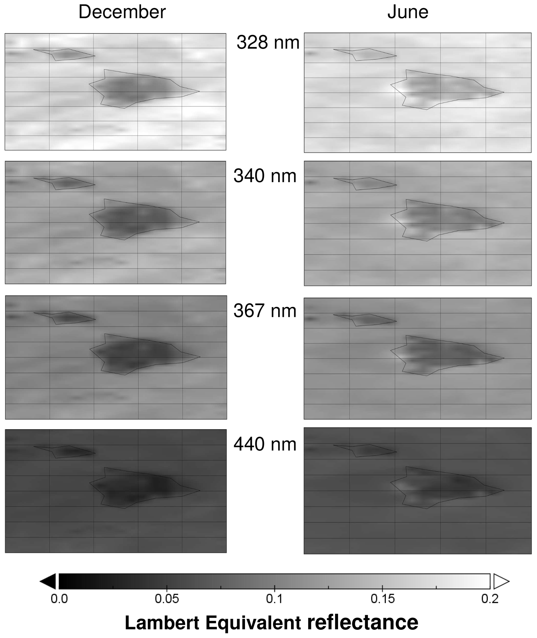
Figure A1 Minimum Lambertian-equivalent albedos over Hawaii derived from TROPOMI observations for December (left) and June (right). Data obtained from the TEMIS database (https://www.temis.nl/, last access: 25 March 2023); see also Tilstra et al. (2021).

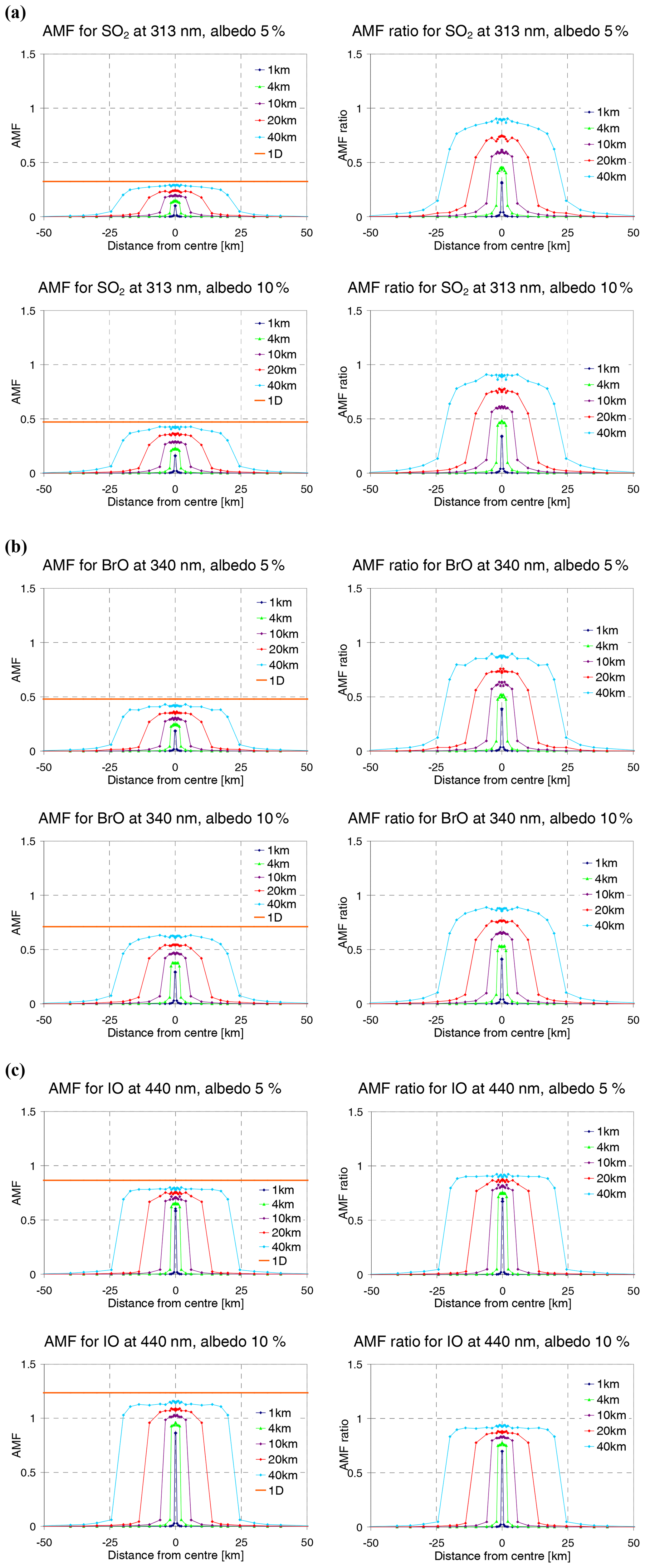
Figure A2 AMFs (left) and corresponding ratios to the 1D AMFs (right) for plume scans in near-nadir viewing geometry (SZA = 0^∘, VZA = 0^∘) for (a) SO₂ at 313 nm, (b) BrO at 340 nm and (c) IO at 440 nm. It is assumed that the satellite scans the plume with a narrow FOV (∼ 0.014^∘). The different colours represent AMFs for plumes at 5–6 km altitude and with different horizontal extensions (from 1 × 1 to 40 × 40 km²). Results are shown for surface albedos of 5 % (as used in general in this study) and 10 %. The ratios of the AMFs for narrow plumes to the corresponding 1D AMFs hardly depend on the surface albedo.

Appendix B: Differential absorption cross sections for the selected trace gases and wavelengths

The following table shows a summary of the differential absorption cross sections used in this study to relate the trace gas SCDs to the corresponding optical depths.

The values were determined by convolution of the original cross section with a Gaussian slit function with a FWHM of 0.5 nm (similar to TROPOMI). In addition to the IO absorption cross section, those of H₂O and NO₂ are also shown, which could also be analysed in the same spectral range around 440 nm. Note that the absorption cross sections depend on temperature. Also, the values from different studies differ, especially for IO and H₂O. Finally, the differential absorption cross sections will depend on the spectral resolution of the instrument. Thus, the values in Table B1 can serve as a useful reference (e.g. in this study) but might differ for other applications.

Table B1 Differential absorption cross sections for the trace gases considered in this study.

Appendix C: Simulation results for different plume altitudes

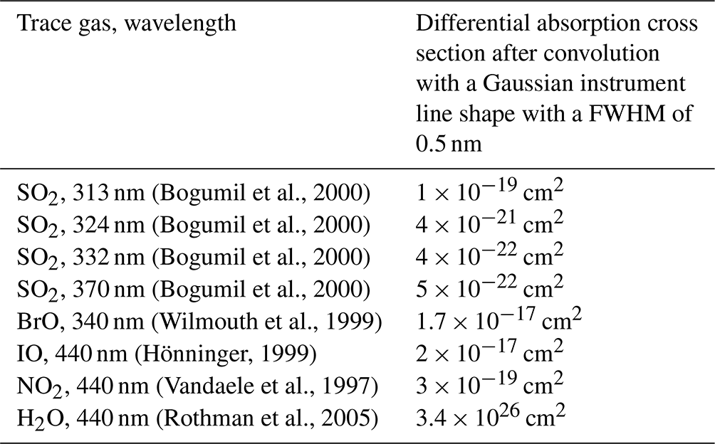
Figure C1 Same as Fig. 6 but for additional plume heights: AMFs for plume scans in near-nadir viewing geometry (SZA = 0^∘, VZA = 0^∘) at different wavelengths. It is assumed that the satellite scans the plume with a narrow FOV (∼ 0.014^∘). The different colours represent AMFs for plumes with different horizontal extensions (from 1 × 1 to 40 × 40 km²).

Figure C2 Same as Fig. 8 but for additional plume heights and wavelengths. Top: retrieved fraction of the plume content as a function of the horizontal plume extension (note the logarithmic scale). Bottom: measured trace gas SCDs (for a 1 × 1 km² pixel). The horizontal dashed lines in (a) indicate the detection limits (see Sect. 2.1). Left: results for a TROPOMI ground pixel; right: results for a large ground pixel of 200 × 200 km². Note that in the case of plume size > ground pixel size, only the fraction of the plume within the ground pixel size is considered. Simulations for VZA = 0 and SZA = 0^∘. The error bars represent the standard deviation calculated from 40 individual simulations.

Figure C3 Same as Fig. 11 but for additional plume heights: AMFs and normalised radiances for plume scans in near-nadir viewing geometry (SZA = 0^∘) for different wavelengths and aerosol contents. The satellite scans the plume with a narrow FOV (∼ 0.014^∘). The different colours represent AMFs for plumes with different horizontal extensions (from 1 × 1 to 40 × 40 km²). The rather low radiance at 313 nm (in spite of the high probability of Rayleigh scattering) is caused by the stratospheric ozone absorption.

Figure C4 Same as Fig. 13 but for additional plume heights: plume scans for SO₂ plumes with different amounts of molecules and different horizontal extensions (for the different SO₂ scenarios; see Table 3). Left: SO₂ VCDs of the plumes; middle: AMFs at 313 nm; right: normalised radiances at 313 nm.

Figure C5 Same as Fig. 14 but for additional plume heights: retrieved fraction of the plume content (top) and SO₂ SCDs (bottom) from TROPOMI measurements at different wavelengths as a function of the plume size and for different amounts of molecules in the plume. The red horizontal line indicates the threshold, above which the operational SO₂ retrieval switches from the standard fit window to the first alternative fit window (at longer wavelengths).

Figure C6 Same as Fig. 15 but for additional plume heights: retrieved fractions of the plume content and SO₂ SCDs for different satellite instruments and for a plume size of 1 × 1 km² as a function of the wavelength. The full symbols represent measurements with SCDs above the detection limit. Note that for the rather large ground pixel sizes of SCIAMACHY and GOME-2, the errors are between 5 % and 10 %.

Appendix D: Effect of the wavelength dependence of the AMF

In this section we quantify the effect of the wavelength dependence of the AMFs for selected representative scenarios by the comparison of the results of two simulations:

• a.

  monochromatic AMFs (only affected by the saturation effect);

• b.

  “true” AMFs (affected by the saturation effect and the wavelength dependence of the AMF).

The true AMFs are calculated in the following way (see also Marquard et al., 2000): first a measured spectrum for a selected SO₂ scenario is simulated at a “high” spectral resolution (∼ 0.22 FWHM, the spectral resolution of the SO₂ cross section). In order to minimise the computational effort for Monte Carlo simulations (and also to minimise the noise), the spectra are calculated in the following way: first a wavelength close to the centre of a SO₂ fit range is chosen. For this wavelength, the radiance is simulated as a function of the absorption cross section. Note that, in order to minimise the noise, the same photon trajectories are used for the simulations with different absorption cross sections. Based on the derived relationship between the radiance and the absorption cross section, a high-resolution spectrum for the selected SO₂ scenario is calculated and convolved by the instrument slit function (here we assume a FWHM of 0.5 nm). In the next step, the simulated spectra are analysed by differential optical absorption spectroscopy (DOAS), similarly to the measured spectra. Finally, the derived SO₂ SCD is divided by the SO₂ VCD (used as input for the respective scenario) to yield the true AMF.

The upper part of Fig. D1 shows the true AMFs derived for the standard fit window around 313 nm and the corresponding monochromatic AMFs for single wavelengths for four different plume scenarios. Additional results for 332 nm are shown in the bottom part of the figure. In addition to the AMFs, the ratios of the monochromatic AMFs and the true AMFs are also shown. For scenarios with high AMFs (monochromatic AMFs > about 0.6), the difference between the monochromatic AMFs and the true AMFs is small (< 10 %), but for smaller AMFs, the difference increases (up to more than 50 % for monochromatic AMFs below about 0.4). In Fig. D2, the ratios of the true AMFs and monochromatic AMFs as a function of the vertical optical depth of the SO₂ absorption are shown. For the same fit window, a similar dependence is found that is almost independent of the SO₂ scenario. However, a different relationship is found for a different fit window indicating the specific spectral patterns of the SO₂ absorption in the different fit windows.

These findings indicate that, for an accurate quantitative assessment, true AMFs for selected plume scenarios and wavelengths have to be individually calculated. Nevertheless, for the wavelengths considered here, the underestimation is < 5 % if the vertical optical depth is below about 2.5 %.

It should also be noted that for scenarios with high optical depth, the “optical definition” of the AMF (Eq. 1) should be used for the interpretation of the measurements. For such cases, the AMFs calculated based on geometric photon trajectories (e.g. box AMFs) will differ from those calculated by Eq. (1) in Puķīte and Wagner (2016).

Figure D1 True AMFs (magenta lines) and monochromatic AMFs (green lines) as a function of the horizontal plume extension for different SO₂ scenarios. Also, the ratios of both AMFs are shown (black lines). The AMFs and AMF ratios depend on the wavelength and the SO₂ amount.

Figure D2 Ratio between true AMFs and monochromatic AMFs as a function of the vertical optical depth of SO₂ in the plume.

Appendix E: Geometric effects for SO₂ (weak) at 313 nm and BrO at 340 nm

Figure E1 AMFs for TROPOMI observations of elevated plumes for different combinations of SZA and VZA. The blue lines show the AMFs for observations with a narrow FOV (∼ 0.014^∘) (right y axis). The bright-blue symbols represent simulations with a TROPOMI FOV (left axis). All simulations are for SO₂ (weak) at 313 nm and plume sizes of 1 × 1 × 1 km³.

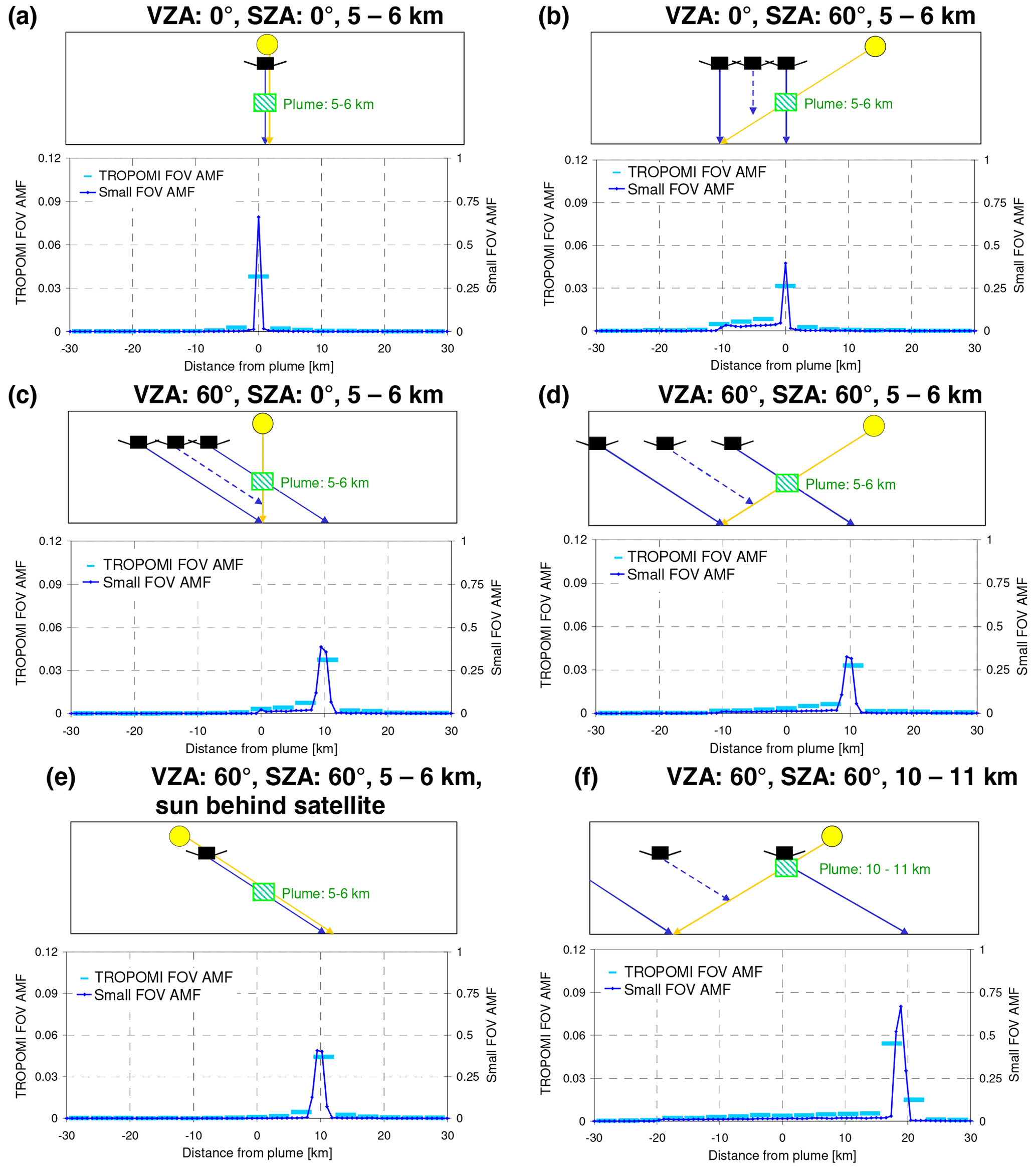
Figure E2 AMFs for TROPOMI observations of elevated plumes for different combinations of SZA and VZA. The blue lines show the AMFs for observations with a narrow FOV (∼ 0.014^∘) (right y axis). The bright-blue symbols represent simulations with a TROPOMI FOV (left axis). All simulations are for BrO at 340 nm and plume sizes of 1 × 1 × 1 km³.