the Creative Commons Attribution 4.0 License.
the Creative Commons Attribution 4.0 License.
 | 27 Jun 2023
Evaluating the consistency between OCO-2 and OCO-3 XCO2 estimates derived from the NASA ACOS version 10 retrieval algorithm
Thomas E. Taylor
Christopher W. O'Dell
David Baker
Carol Bruegge
Albert Chang
Lars Chapsky
Abhishek Chatterjee
Cecilia Cheng
Frédéric Chevallier
David Crisp
Lan Dang
Brian Drouin
Annmarie Eldering
Liang Feng
Brendan Fisher
Dejian Fu
Michael Gunson
Vance Haemmerle
Graziela R. Keller
Matthäus Kiel
Thomas Kurosu
Alyn Lambert
Joshua Laughner
Richard Lee
Junjie Liu
Lucas Mandrake
Yuliya Marchetti
Gregory McGarragh
Aronne Merrelli
Robert R. Nelson
Greg Osterman
Fabiano Oyafuso
Paul I. Palmer
Vivienne H. Payne
Robert Rosenberg
Peter Somkuti
Gary Spiers
Cathy To
Brad Weir
Paul O. Wennberg
Shanshan Yu
Jia Zong
The version 10 (v10) Atmospheric Carbon Observations from Space (ACOS) Level 2 full-physics (L2FP) retrieval algorithm has been applied to multiyear records of observations from NASA's Orbiting Carbon Observatory 2 and 3 sensors (OCO-2 and OCO-3, respectively) to provide estimates of the carbon dioxide (CO2) column-averaged dry-air mole fraction (XCO2). In this study, a number of improvements to the ACOS v10 L2FP algorithm are described. The post-processing quality filtering and bias correction of the XCO2 estimates against multiple truth proxies are also discussed. The OCO v10 data volumes and XCO2 estimates from the two sensors for the time period of August 2019 through February 2022 are compared, highlighting differences in spatiotemporal sampling but demonstrating broad agreement between the two sensors where they overlap in time and space. A number of evaluation sources applied to both sensors suggest they are broadly similar in data and error characteristics. Mean OCO-3 differences relative to collocated OCO-2 data are approximately 0.2 and −0.3 ppm for land and ocean observations, respectively. Comparison of XCO2 estimates to collocated Total Carbon Column Observing Network (TCCON) measurements shows root mean squared errors (RMSEs) of approximately 0.8 and 0.9 ppm for OCO-2 and OCO-3, respectively. An evaluation against XCO2 fields derived from atmospheric inversion systems that assimilated only near-surface CO2 observations, i.e., did not assimilate satellite CO2 measurements, yielded RMSEs of 1.0 and 1.1 ppm for OCO-2 and OCO-3, respectively. Evaluation of uncertainties in XCO2 over small areas, as well as XCO2 biases across land–ocean crossings, also indicates similar behavior in the error characteristics of both sensors. Taken together, these results demonstrate a broad consistency of OCO-2 and OCO-3 XCO2 measurements, suggesting they may be used together for scientific analyses.
- Article
(15920 KB) - Full-text XML
- BibTeX
- EndNote


Estimates of the column-averaged carbon dioxide (CO2) dry-air mole fraction (XCO2) derived from global space-based measurements can be assimilated into atmospheric inversion systems to quantify CO2 fluxes associated with both natural and anthropogenic sources and sinks (Gurney et al., 2002). However, these estimates must have both high precision and accuracy due to the long atmospheric lifetime of CO2 (Archer et al., 2009) and the high background concentrations (≈ 415 parts per million by volume, ppm, in 2022) such that even the most intense sources and sinks produce only small (≈ 1 ppm) changes in XCO2 (Miller et al., 2007).
The Orbiting Carbon Observatory 2 and 3 missions, OCO-2 and OCO-3, respectively, referred to collectively as OCO in this document, are NASA's primary operating assets for monitoring CO2 concentrations from space. Both of these instruments measure reflected solar radiation at high spectral resolution in specific narrow spectral bands in the near-infrared and shortwave infrared regions (NIR and SWIR, respectively), where molecular oxygen (O2) and CO2 absorb sunlight. A variety of physics-based algorithms and sources of prior information are required to convert the measured spectra into estimates of XCO2 in a series of steps. First, the individual soundings are geolocated and then radiometrically and spectrally calibrated. Then, these products are pre-screened to filter out scenes contaminated by clouds and heavy aerosol loading. A retrieval is then performed to estimate XCO2 from the geolocated and calibrated radiances. Finally, a post-processing step is applied that quality-screens the retrieval output and applies an empirically based bias correction to the XCO2 concentrations. Although estimates of solar-induced chlorophyll fluorescence (SIF) are also provided from OCO-2 and OCO-3 measurements, the focus of this paper is on the XCO2 estimates. Readers are referred to Doughty et al. (2022) for an overview of the OCO SIF products.
Space-based measurements from OCO-2 and OCO-3 have already been successfully used to quantify CO2 sources and sinks at global (e.g., Crowell et al., 2019; Peiro et al., 2022; Byrne et al., 2023), regional (e.g., Palmer et al., 2019; Byrne et al., 2021; Philip et al., 2022), and even local and/or urban scales (e.g., Lei et al., 2021; Kiel et al., 2021; Nassar et al., 2022). However, biases and random errors in the XCO2 estimates relative to reference measurements persist, even after application of bias correction and filtering. These biases and random errors are associated with multiple factors, such as instrument measurement noise, uncertainties in instrument calibration, error in CO2 and O2 gas absorption cross sections, complications in accurately representing aerosols and surface characteristics in the retrieval, and lack of accurate knowledge of the prior estimates of the atmospheric state that are used in the retrieval algorithm (Connor et al., 2016; Kulawik et al., 2016; Hobbs et al., 2017; Kulawik et al., 2019). Numerous studies have demonstrated that small, but regionally coherent, biases in CO2 concentrations can result in flux estimate errors (e.g., Chevallier et al., 2005, 2007, 2014; Basu et al., 2013; Feng et al., 2016). It is therefore essential to quantify, as well as possible, the remaining biases present in the satellite XCO2 products.
The paper is organized as follows: the OCO instruments, spectral measurements, and calibration are reviewed in Sect. 2. Section 3 discusses updates to the v10 L2FP retrieval algorithm and other components of the data processing pipeline. In Sect. 4, the OCO-2 and OCO-3 v10 XCO2 data volumes are analyzed for the overlapping time period of August 2019 through February 2022, while Sect. 5 compares the XCO2 estimates from the two sensors. Section 6 compares the satellite XCO2 estimates from both sensors to XCO2 estimates derived from the Total Carbon Column Observing Network (TCCON), atmospheric inversion systems (models), and small areas and coastal crossings. A summary of the findings is presented in Sect. 7. A deeper examination of the full OCO-2 v10 record, which spans more than 7 years, is provided in Appendix A. Finally, in Appendix B, several aspects of the OCO-3 v10 dataset are explored in detail, including the application of a time-dependent correction to the OCO-3 v10 XCO2 estimates to correct a calibration artifact using a set of soundings collocated with OCO-2.
There are many similarities between the OCO-2 and OCO-3 sensors, as the latter was built as a flight spare for the former. Both are three-channel grating spectrometers with a common telescope used to direct reflected solar radiation from the field of view through a dispersion grating onto a focal plane array (FPA). The FPA electronics convert analog signals into measured digital numbers (DNs). Predetermined calibration information is used to convert DNs into radiances (photons s−1 m−2 sr−1 µm−1) in the three spectral channels: (i) the oxygen A band centered at 0.765 µm, (ii) a weak CO2 band centered at 1.61 µm, and (iii) a strong CO2 band centered at 2.06 µm, referred to as the ABO2, WCO2, and SCO2, respectively, all with high spectral resolving power ( > 17 000) and 1016 spectral channels. A single OCO measurement frame contains eight along-slit “footprints”, which are acquired at 3 Hz, yielding 24 individual soundings per second. The exact footprint size of each OCO-2 sounding varies by observation mode and latitude but is of the order of 1.3 km cross-track and 2.25 km along-track (2.9 km2) near-nadir viewing. The orbit altitude of OCO-3 aboard the International Space Station (ISS) is lower than that of OCO-2 (≈ 400 and ≈ 705 km for OCO-3 and OCO-2, respectively), necessitating an enlargement of the instrument's field of view from 0.8 to 1.8∘ in order to maintain a similar footprint size. Even so, OCO-3 footprints are typically slightly larger, at 1.6 km cross-track by 2.2 km along-track (3.5 km2).
OCO-2 began science operations in September 2014 (Crisp et al., 2017; Eldering et al., 2017). It flies in a sun-synchronous polar orbit on a dedicated satellite bus in the afternoon constellation, i.e., A-train constellation (L'Ecuyer and Jiang, 2010), which has a local overpass time of approximately 13:36 and a 16 d orbit repeat cycle. OCO-2 science measurements are made in one of three observation modes: (i) down-looking nadir (ND), (ii) sun glint (GL), or (iii) target (TG). For routine science observations, a full dayside orbit is acquired in one of the two primary observation modes (nadir or glint) in an alternating fashion. However, for orbits that pass largely over ocean, the satellite orients the instrument to view the sun's specular glint spot, which maximizes the signal over water (Miller et al., 2007). In addition, a small number (order 30) of predetermined target sites are viewed as conditions allow. Most of the targeted observations are collected over Total Carbon Column Observing Network (TCCON) stations, whose up-looking observations are used to validate the OCO-2 XCO2 estimates (Wunch et al., 2011a, 2017). Other targets include surface calibration sites (e.g., Bruegge et al., 2019), large urban areas (e.g., Rißmann et al., 2022), and power plants (e.g., Nassar et al., 2017).
OCO-3 began science operations in August 2019 (Taylor et al., 2020). The OCO-3 instrument is mounted as an external payload on the Japanese Experimental Module – Exposed Facility (JEM-EF) aboard the ISS. The ISS flies in a precessing orbit with a varying time-of-day local overpass across a 63 d illumination cycle. To provide agile pointing from the ISS, a two-axis pointing mirror assembly (PMA) was added to the fore optics of OCO-3 (Eldering et al., 2019). For routine science observations, OCO-3 acquires measurements in nadir mode over land and glint mode over large water bodies. A much larger set of target observations is possible compared to OCO-2 due to the more up-to-date onboard electronics control system and the rapid repointing allowed by the PMA. In addition, a new observation mode called snapshot area mapping (SAM) allows the instrument to compile contiguous images as large as 80 by 80 km2 over sites of interest such as mega-cities, power plants, volcanoes, flux towers, and field campaigns. The spatially contiguous nature of the SAMs is already showing tremendous promise for carbon cycle science (e.g., Kiel et al., 2021; Wu et al., 2022; Roten et al., 2022; Nassar et al., 2022) and for investigating sources of bias within the L2FP retrieval (Bell et al., 2023).
The precision and accuracy requirements for OCO-2 and OCO-3 were originally applied to regional scales, roughly defined as 10∘ latitude by 10∘ longitude. Early observation system simulation experiments (OSSEs) indicated that XCO2 precision and accuracy better than 1 ppm (less than 0.25 %) are needed at this scale to constrain typical natural and anthropogenic sources and sinks of CO2 (Miller et al., 2007). In practice, the spatial scale for precision and accuracy requirements is determined by the distribution of the validation reference measurements. This is defined by the approximately 24 TCCON stations and a comparable number of EM27/SUN and Aircore stations distributed over the globe. The system performance on finer scales has also been assessed through comparisons with data collected by aircraft campaigns, e.g., ACT-America (Bell et al., 2020) and ATom (Kulawik et al., 2019), as well as multi-instrument EM27/SUN campaigns (Rißmann et al., 2022).
The precision and accuracy requirements place strict demands not only on the instrument sensitivity, but also on its calibration and the accuracy of the retrieval algorithm. Both OCO-2 and OCO-3 were radiometrically calibrated prior to launch using integrating sphere sources calibrated with respect to the National Institute of Standards and Technology (NIST) reference standards. Observations of the integrating spheres yielded pre-launch gain coefficients used to convert measured digital numbers into radiances. The radiometric calibration of OCO-2 and OCO-3 is frequently updated in-flight through the use of onboard calibration systems (Crisp et al., 2017; Keller et al., 2022), which are analyzed to update Ancillary Radiometric Products (ARPs) covering 3 to 7 d; gain degradation coefficients are provided to correct radiances based on pre-launch gains.
For OCO-2, in-flight updates to the pre-launch calibration are derived from observations of the sun through a transmissive diffuser and from its primary onboard lamp. While the sun observations track the overall change in instrument response with time, lamp observations provide corrections of relative changes in the response of the individual samples, which are comprised of 20 detector pixels each (see Fig. 2 of Crisp et al., 2017, for the readout scheme). Lunar observations taken throughout the mission have been used to track and account for the degradation of the solar diffuser. Details of the pre-flight and on-orbit calibration of OCO-2 Level 1b (L1b) can be found in Rosenberg et al. (2017), Lee et al. (2017), Crisp et al. (2017), and Marchetti et al. (2019). In general, the instrument calibration and the full-physics retrieval algorithm for OCO-2 have reached relatively mature states. For example, updates to the OCO-2 v10 calibration algorithms used to produce calibrated L1b spectra were limited to an improved treatment of radiometric degradation using lunar calibration observations, a small refinement in the spectral dispersion coefficients, and the identification of additional spectral sample outliers (Crisp et al., 2021).
Keller et al. (2022) describe the current state of the calibration for the L1b OCO-3 v10 data products. OCO-3, unlike OCO-2, cannot view the sun from the ISS, making solar calibration impossible (Rosenberg et al., 2020). Therefore, compared to OCO-2, more emphasis has been placed on the internal lamp calibration system, which is comprised of three tungsten halogen lamps and a reflective diffuser. The three calibration lamps are illuminated with different cadences and thus age at different rates. For v10 L1b, an algorithm was developed to use information from all three lamps with the goal of mitigating lamp aging while still allowing changes in instrument response to be tracked with the necessary temporal resolution. This is particularly important for OCO-3, as it has exhibited significant, abrupt changes in its overall instrument response. In addition, an update was made to the OCO-3 stray light model used for v10 L1b to account for spatial variability on the detectors. More detail is provided in Sect. 2.1 of the OCO-3 v10.4 data quality statement (Chatterjee et al., 2022). Because of initial difficulties in reducing geolocation errors for OCO-3, plans to perform lunar calibration, intercomparison of L1b radiances with OCO-2, and vicarious calibration using the Railroad Valley Playa were delayed. These are now all underway and will inform the in-flight calibration for the next OCO-3 product version. Additional OCO-3 calibration details are contained in the L1b Algorithm Theoretical Basis Document (ATBD) (Crisp et al., 2021).
Beginning with the geolocated and calibrated L1b spectra, the ACOS pipeline consists of three distinct steps to produce the final estimates of XCO2. First, due to the computational demands of the L2FP retrieval algorithm, which requires about 5 min per sounding on a single processor, and the inability to reliably estimate XCO2 in the presence of clouds and heavy aerosol loadings, a pre-screening step is performed to identify and remove these soundings (Taylor et al., 2016). The soundings that are identified as likely to yield good-quality results are then input to the ACOS Level 2 full-physics (L2FP) retrieval algorithm, which utilizes a Bayesian optimal estimation framework to derive estimates of XCO2 by combining information from the L1b spectra with prior information about the state of the atmosphere and measurement geometry (Rodgers, 2004; Connor et al., 2008; O'Dell et al., 2012). In a post-processing step, each sounding that successfully converges within the L2FP is assigned either a good or bad quality flag based on a set of empirically derived filters. Furthermore, an empirical, parametric bias correction, derived from comparisons with multiple truth proxies, is applied to each sounding (O'Dell et al., 2018). The quality-filtered and bias-corrected XCO2 estimates are included in the L2 Lite files, which also contain essential retrieval, time, and geometry information. A brief summary of recent changes specific to v10 is provided in Sect. 3.1.
3.1 Level 2 full-physics retrieval algorithm updates for v10
ACOS v10 is the fourth major reprocessing of the OCO-2 record, which began with the v6 release in December 2014, followed by v7 in 2015 and v8 in 2017 (O'Dell et al., 2018). The v9 XCO2 product, released in 2018, was a post-processing-only effort to correct XCO2 errors introduced by a small error in the instrument boresight pointing and geolocation (Kiel et al., 2019). Since there were no changes to the L2FP code from v8 to v9, for the remainder of this document the nomenclature “v8/9” will be used to refer to the previous version of the algorithm. For OCO-3, the v10 XCO2 product is only the second public release. It is a substantial improvement over the first release, vEarly, which employed the ACOS v10 algorithm but had significant instrument calibration and geolocation errors and was quality-filtered and bias-corrected against a very short data record of only a few months (Taylor et al., 2020). Table 1 summarizes the four substantial changes that were made to the ACOS L2FP retrieval algorithm from v8/9 to v10. More detail can be found in the v10 L2FP ATBD (Crisp et al., 2020).
Table 1Updates to the ACOS L2FP retrieval algorithm from v8/9 to v10.
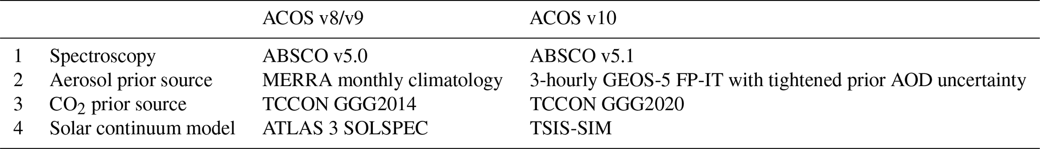
Each new release of ACOS uses the latest gas absorption coefficient (ABSCO) tables produced at NASA's Jet Propulsion Laboratory (JPL). For v10, the ABSCO tables were updated from v5.0 (Oyafuso et al., 2017) in ACOS v8/9 to ABSCO v5.1 in ACOS v10 (Payne et al., 2020). The most significant changes occurred in the ABO2 spectral band (Drouin et al., 2017; Payne et al., 2020) related to consistency between oxygen line shapes and collision-induced absorption. This update yielded reduced spatial variability of the bias between the L2FP retrieved surface pressure and the prior value from 3.3 hPa in v9 to 2.8 hPa in v10. ABSCO v5.1 also includes an update to the water vapor continuum model, which affects the WCO2 and SCO2 spectral bands.
A second important change between ACOS v8/9 and v10 was an update of the prior values adopted for aerosol types, optical depths (AODs), vertical distribution, and uncertainties. In previous versions, the aerosol priors were compiled from a monthly climatology derived from the NASA Goddard Modeling and Assimilation Office (GMAO) Modern-Era Retrospective analysis for Research and Applications version 2 (MERRA-2) product (Rienecker et al., 2008, 2011; Gelaro et al., 2017). For v10, these monthly aerosol priors were replaced with daily estimates derived from the GEOS-5 Forward Product for Instrument Teams (FP-IT) product. Furthermore, the AOD prior variance (expressed in log(AOD)) was reduced from 2 to 0.5 in v10. These changes led to significant improvements in both retrieved aerosol values and estimates of XCO2 from OCO-2, especially in aerosol-laden regions. Full details on the v10 aerosol formulation, including tests on its efficacy, are provided in Nelson and O'Dell (2019) and Sect. 3.3.2.3 of Crisp et al. (2020).
A third significant change from v8/9 to v10 was replacing the source of the CO2 prior profiles from that developed by the TCCON team for use in the GGG2014 algorithm (Wunch et al., 2015) to the newest version used in GGG2020 (Laughner et al., 2023). A complete description of the calculation of the v10 CO2 priors is provided in Sect. 3.3.2.1 of the L2FP ATBD (Crisp et al., 2020). In short, the priors are calculated from a scaling of the NOAA monthly averaged flask values (Lan et al., 2022) measured at the Mauna Loa and American Samoa sites to individual sounding dates and locations. The tropopause altitude is derived from data contained in the 3-hourly GOES-FPIT meteorology, which has a nominal 1 d lag and provides diagnosed potential vorticity, allowing for better representation of latitudinal CO2 transport in the stratosphere. A previous study using measurements from the Japanese Greenhouse Gases Observing Satellite (GOSAT; Kuze et al., 2009) processed with the ACOS v9 L2FP retrieval showed that a correction to account for the difference in the CO2 prior from v8/9 to v10 yielded a global mean adjustment in XCO2 of approximately 0.2 ppm, with 95 % of changes falling between −0.1 and +0.5 ppm (Taylor et al., 2022).
The last significant change to the v10 L2FP was replacement of the solar continuum model used to simulate the top-of-atmosphere (TOA) solar spectrum. For the OCO missions, a high-resolution TOA solar spectrum is derived by combining a high-spectral-resolution solar transmission spectrum for solar Fraunhofer lines with an observed, low-spectral-resolution TOA solar spectrum. The solar transmission spectrum is derived from an empirical solar line list (Toon, 2014). In earlier versions of the L2FP model, the solar continuum was derived to fit the ATLAS 3 SOLSPEC measurements (Thuillier et al., 2003) when the OCO solar spectrum was convolved with the SOLSPEC spectral response function (SRF). For v10, this continuum was replaced by one derived to fit new measurements from the Total Solar Irradiance Sensor (TSIS) Spectral Irradiance Monitor (SIM) aboard the ISS (Richard et al., 2020) when convolved with the TSIS-SIM SRF. The new solar model reduced the solar continuum values by ≈ −1.3 %, −3.0 %, and −6.5 %, in the ABO2, WCO2, and SCO2 spectral bands, respectively. These results are consistent with the more recently derived TSIS-1 Hybrid Solar Reference Spectrum (Coddington et al., 2021). L2FP tests indicated that these changes had a minimal impact on XCO2 estimates. This is most likely because the solar flux differences were relatively small in the ABO2 channel, which is most sensitive to the accuracy of the solar illumination and absolute radiometric calibration. However, even these small differences shifted the retrieved surface pressures by ≈ −0.2 hPa for land and ≈ +0.2 hPa for ocean soundings, which has a small impact on the bias correction.
3.2 Preprocessor and sounding selection for v10
The ACOS software includes two preprocessors to flag soundings that are likely to fail to converge in the full-physics retrieval due to cloud and aerosol: the A-band preprocessor (ABP) (Taylor et al., 2012, 2016) and the IMAP-DOAS preprocessor (IDP) (Frankenberg et al., 2005; Taylor et al., 2016). For v10, an update was made to the ABP state vector to include a zero-level offset to the calculated top-of-atmosphere radiances to account for instrument stray light and SIF. The v10 ABP uses v5.1 ABSCO to be consistent with the L2FP retrieval. To accommodate changes to the ABSCO and L1b, updates were made to tune the ABP surface pressure vs. solar zenith angle and chi-squared vs. signal-to-noise ratio parameterizations, both of which are used as individual filters to determine scenes contaminated by clouds and aerosols as first described in Taylor et al. (2012) for application to GOSAT and more recently in Taylor et al. (2016) as applied to OCO-2.
The IDP algorithm serves two purposes in the ACOS pipeline: (i) single-band retrievals of CO2 and H2O are used for cloud screening, and (ii) the ABO2 spectral band is used to estimate SIF (Frankenberg et al., 2012; Doughty et al., 2022). For v10, no changes were made to the IDP. In fact, the code has remained unaltered for many versions, including use of the older v4.2 ABSCO (Drouin et al., 2017).
Table 2Sounding selection criteria for OCO-2 and OCO-3 v10. Soundings are categorized as either land (land fraction ≥ 80 %), water (land fraction ≤ 20 %), or indeterminate (20 % < land fraction < 80 %). N/U: not used. N/P: not processed. In addition to the criteria defined in the table, all soundings must have a “sounding quality flag” of 0.
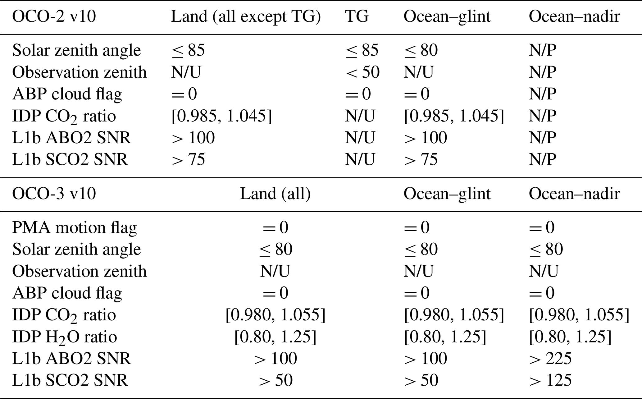
The sounding selection strategy, which determines if a sounding should be run through the L2FP, remains roughly consistent for v10 compared to previous versions. Details are provided in Table 2. For both sensors, the single difference between land and ocean–glint selection criteria is that for OCO-2, the solar zenith angle (SZA) cutoff is slightly more strict at 80∘ for ocean–glint compared to 85∘ for land. For OCO-3, the SZA cutoff is 80∘ for both land and ocean–glint. For OCO-2 v10, target-mode observations were filtered using the satellite observation angle to remove soundings more oblique than 50∘. This criterion was removed for OCO-3 target (and SAM) observations so that the same set of selection criteria is used for all land observations. Because there is minimal information content in ocean–nadir measurements due to a low signal-to-noise ratio (SNR), no ocean–nadir soundings were selected for OCO-2 v10. However, the early part of the OCO-3 record contains a large fraction of ocean–nadir observations prior to tuning of the PMA. To maximize the selection of potentially good-quality soundings, the L1b SNR filters in both the ABO2 and SCO2 spectral bands were relaxed. However, the scientific merit of the ocean–nadir observations is as of yet undetermined, and therefore ocean–nadir soundings are not considered further in this work.
3.3 Postprocessing: quality filtering and bias correction for OCO v10 XCO2 estimates
All selected soundings, as described in Sect. 3.2 are subsequently processed by the L2FP retrieval, which primarily estimates XCO2. Soundings that converge (typically ≈ 85 %–90 % of the attempts), are reported in the L2 Standard product files (L2Std), which are organized into granules that typically include full orbits or partial orbits, yielding about 15 files per day. The L2Std files are in HDF5 format and are about 20 MB each (≈ 300 MB per day). Next, a post-processing step assigns to each sounding a binary quality flag (QF = 0 indicates the best data), as well as a bias correction adjustment to XCO2 (O'Dell et al., 2018). The results are aggregated into daily output L2 Lite XCO2 files. Lite files are in NetCDF format and are typically about 50–70 MB each. It is highly recommended that only the good-quality (QF = 0) soundings contained in the L2 Lite XCO2 product be used in global- and regional-scale studies, although local-scale studies may benefit from the use of some of the lower-quality (QF > 0) soundings.
3.3.1 Quality filtering and bias correction truth proxies
The quality filtering and bias correction procedure requires XCO2 truth proxies with which to compare the retrieved estimates. The term truth proxies is used to describe sources of data which can be used as an independent estimate of the atmospheric CO2 abundance. For OCO v10, three truth proxies were used. The first comprised estimates of XCO2 derived from TCCON measurements. Table 3 provides a list of TCCON stations, locations, operational ranges, and data citations. Although TCCON XCO2 estimates have relatively high precision and accuracy while providing good temporal coverage at most sites, they are very limited in spatial extent, especially outside the northern midlatitudes.
Kivi et al. (2020)Wunch et al. (2018)Deutscher et al. (2017)Notholt et al. (2019)Hase et al. (2015)Te et al. (2014)Warneke et al. (2014)Sussmann and Rettinger (2018a)Sussmann and Rettinger (2018b)Wennberg et al. (2017a)Morino et al. (2018c)Wennberg et al. (2016)Goo et al. (2017)Morino et al. (2018a)Petri et al. (2020)Iraci et al. (2016)Wennberg et al. (2017b)Wennberg et al. (2017b)Wennberg et al. (2015)Shiomi et al. (2014)Blumenstock et al. (2017)Morino et al. (2018b)Feist et al. (2017)Griffith et al. (2014a)De Mazière et al. (2017)Griffith et al. (2014b)Pollard et al. (2017)Table 3TCCON stations used in the quality filtering and bias correction of OCO-2 and OCO-3 v10. Sites used only for OCO-2 are indicated with a in the first column. Sites located on an island are indicated with b in the second column.
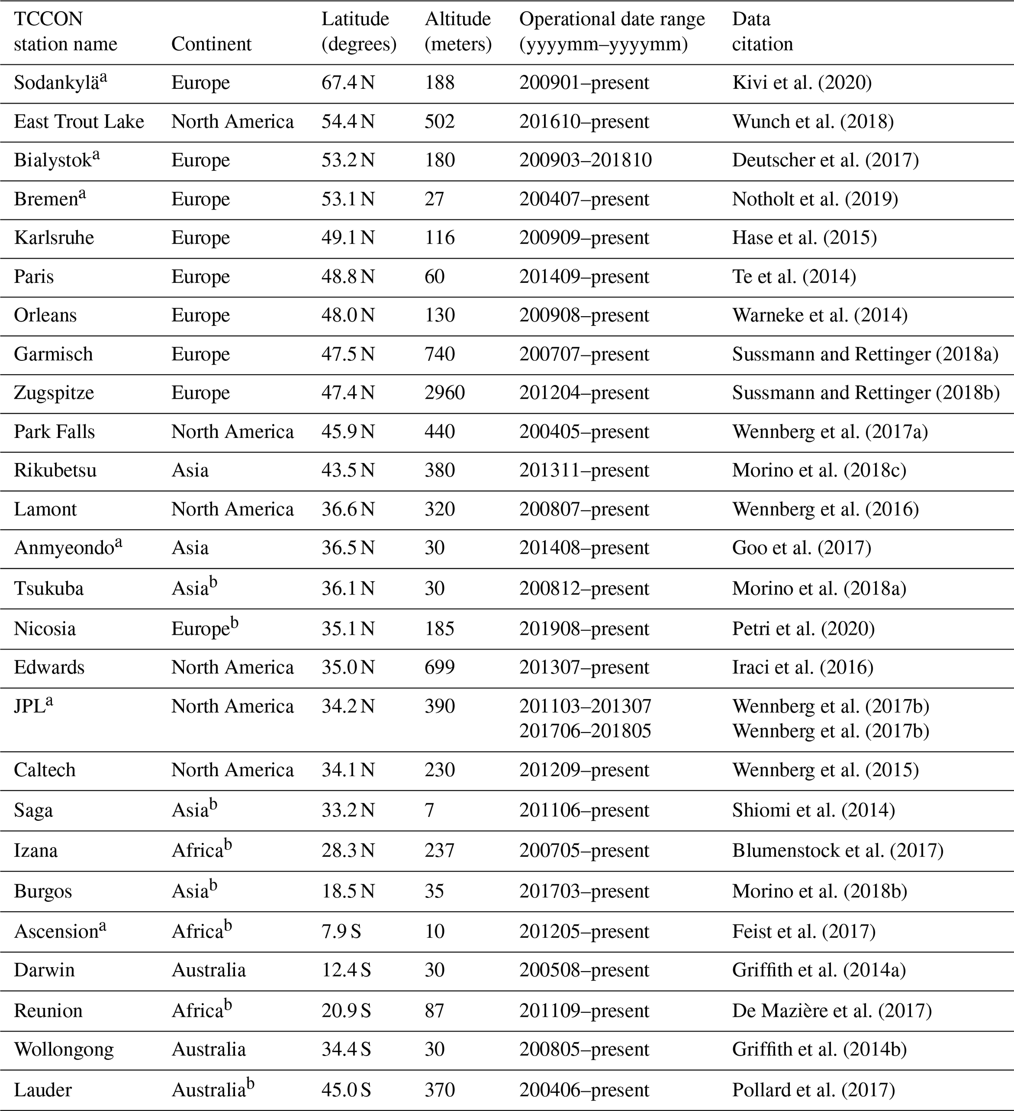
Table 4Names, institutions, and citations of the atmospheric inversion systems used in the quality filtering, bias correction, and XCO2 evaluation of OCO v10.
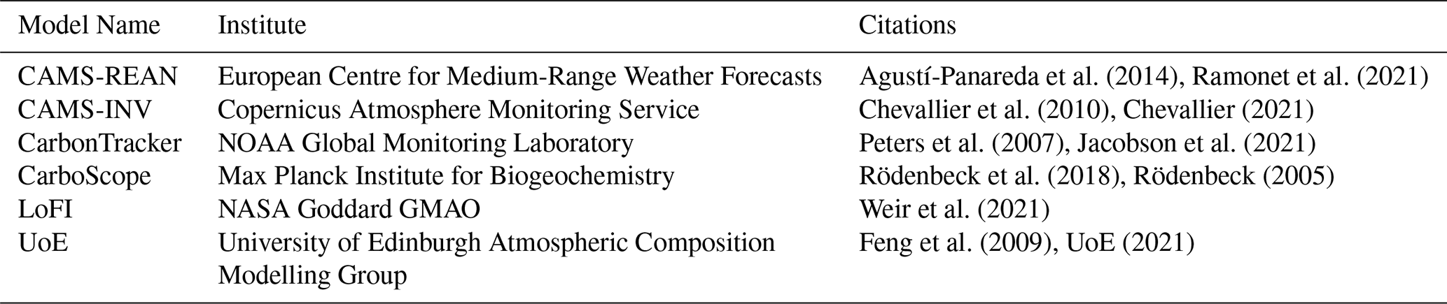
Table 5Characteristics of models used for quality filtering, bias correction, and evaluation of OCO v10. The notation n/a indicates not applicable.
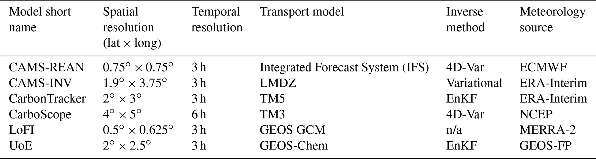
Table 6Model versions used for the quality filtering, bias correction (indicated by an asterisk ∗), and XCO2 evaluation of OCO v10. The notation n/a means not applicable.
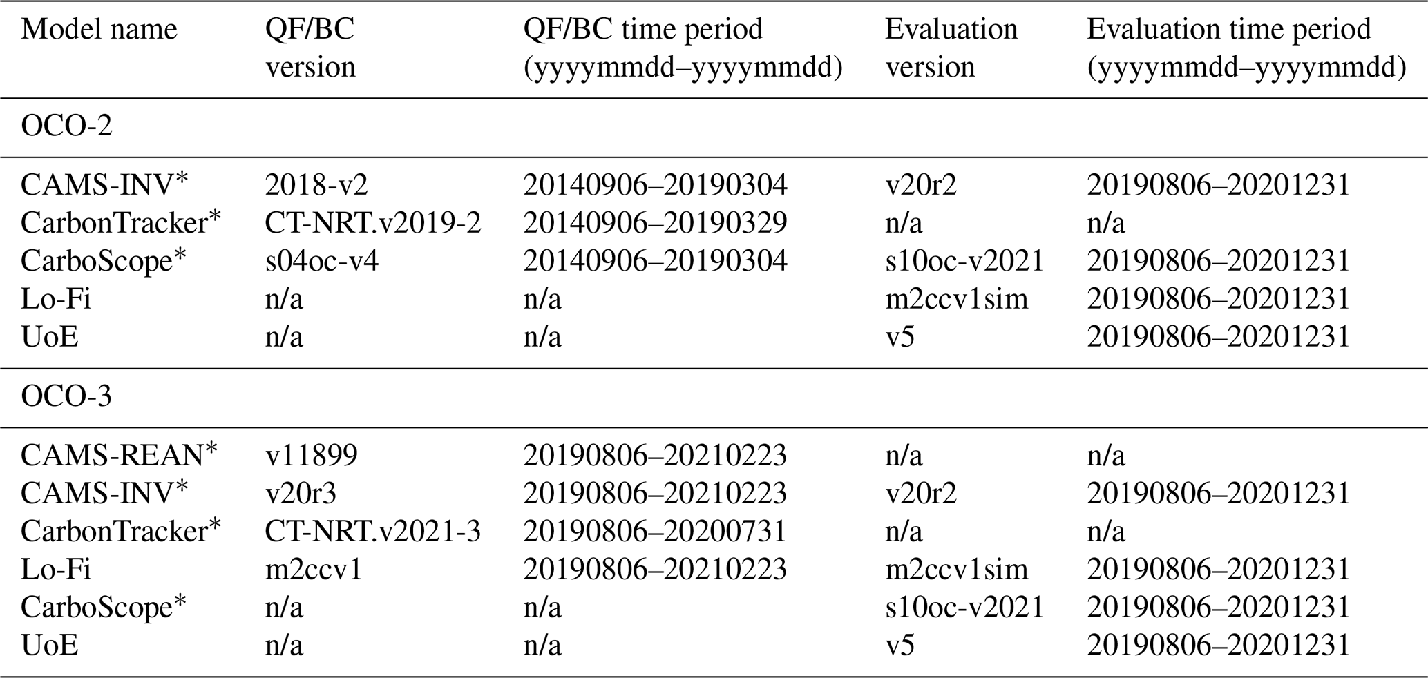
To augment the sparse spatial coverage of TCCON, atmospheric inversion models are used in the OCO XCO2 quality filtering and bias correction process to provide full global coverage (O'Dell et al., 2018). For ACOS v10, the median XCO2 was derived from the four-dimensional (4D) CO2 fields of models that assimilated only in situ CO2 data. To ensure consistency in the models, for each OCO sounding, only the models with XCO2 that deviated by less than ±1.5 ppm from the initial median value were retained. Furthermore, soundings were excluded if more than one of the models had been rejected or if the standard deviation amongst the valid models was > 1 ppm. Tables 4, 5, and 6 provide information about the suite of models. An asterisk is used in Table 6 to identify the specific models and data versions used in the quality filtering and bias correction procedure: three for OCO-2 and four for OCO-3 v10. Some of the same models were also used in the XCO2 evaluation, but using a different model data version and a different evaluation period. A few of the models were used only for the XCO2 product evaluation.
An averaging kernel correction was applied to both the TCCON and the model XCO2 values to account for differences in the vertical profiles compared to the ACOS prior. The general form of the equation is
Here, hi is the pressure weighting function on the i=1…20 ACOS model levels, defined as the pressure intervals assigned to the state vector normalized by the surface pressure and corrected for the presence of atmospheric water vapor. See Appendix A of O'Dell et al. (2012) for details. The vector a is the CO2 column averaging kernel, which relates the sensitivity of the retrieved CO2 to the true atmospheric state of CO2 at each vertical level, as described in Connor et al. (2008). The vector um is the retrieved TCCON or model profile of CO2, linearly interpolated from the native vertical resolution to the 20 ACOS levels. The vector ua is the ACOS prior profile of CO2. Generally the averaging kernel corrections are on the order of 0.5 ppm or less.
Finally, a third truth proxy for training the v10 quality filtering and bias correction was the “small area approximation” (SAA). Each small area is a collection of OCO XCO2 soundings over < 100 km sections within single orbits, for which, in the absence of strong localized sources, the real uncertainty in XCO2 is expected to be well under 0.1 ppm (Worden et al., 2017). A median value of each small area provides a truth proxy to which each sounding in the small area can be compared. While small areas are not suitable for determining large-scale biases in the satellite data, they provide a measure of the uncertainty in the XCO2 estimates due to both instrument noise and systematic errors that act on smaller scales. This “actual” uncertainty can be compared to the “theoretical” uncertainty derived from the L2FP retrieval and stored in the L2Lite files as xco2_uncertainty. For the v10 quality filtering and bias correction training, approximately 750 × 103 and 280 × 103 small areas were identified for OCO-2 and OCO-3, respectively.
3.3.2 Quality filtering and bias correction methodology
Details of the OCO quality filtering procedure are described in Sect. 4.2 of Kiel et al. (2019) for the OCO-2 v9 product and in Sect. 6.2 of Taylor et al. (2020) for OCO-3 vEarly. Here, the method is summarized and differences in the v10 implementation for OCO-2 and OCO-3 are highlighted. In short, the quality filtering procedure assigns to each sounding in the L2Std XCO2 product a good (QF = 0) or bad (QF = 1) binary quality flag based on comparison to truth proxies. A number of retrieval parameters (32 for OCO-2 v10 and 30 for OCO-3 v10.4) are assigned threshold cutoff values, outside which a sounding is considered unreliable, although all soundings in the L2Std product are retained in the L2 Lite XCO2 files. The selected variables and their threshold values can be found in Sect. 3.2.4 of the OCO-2 v10 Data User Guide (DUG) (Osterman et al., 2020) and Sect. 5.1.2 of the OCO-3 v10.4 DUG (Payne et al., 2022). Training for the quality filtering and bias correction procedure takes place on a quick test set (QTS), which is an intelligently selected subset of approximately 5 % of the full OCO data record that is available at the time of the training.
The methodology for the empirical bias correction of the XCO2 estimates was first described in Wunch et al. (2011b) and later in more detail by O'Dell et al. (2018), wherein the fundamental equation for OCO is defined as
Here, CP is the mode-dependent parametric bias, CF is a mode- and footprint-dependent bias for each of the eight footprints, and C0 represents a mode-dependent global scaling factor. Bias correction coefficients are derived using only soundings that have been assigned a good quality flag. Many details related to the v10 quality filtering and bias correction can be found in the DUGs (Osterman et al., 2020; Payne et al., 2022).
For ACOS OCO-2 v10, the selected bias correction parameters are similar to those used in previous versions. For land, the parameters are (i) a term related to the deviation in the retrieved CO2 profile from the prior, “CO2 grad del”, (ii) the difference between the elevation-adjusted retrieved surface pressure and the prior surface pressure, dPfrac, (iii) the combined aerosol optical depth (AOD) of coarse-mode particles, , and (iv) the AOD of fine-mode particles, AODfine. Ocean retrievals use two terms: (i) CO2 grad del and (ii) the difference between the retrieved and prior surface pressure in the SCO2 band, dPSCO2. The bias correction is very similar for OCO-3 v10, with the exception that the coefficients are slightly different, and over land, the AODfine term has been replaced with criteria based on the retrieved albedo in the weak CO2 channel.
Table 7Summary of the OCO-2 and OCO-3 v10 quality filtering (QF) and bias correction (BC) results versus the individual XCO2 truth proxies.
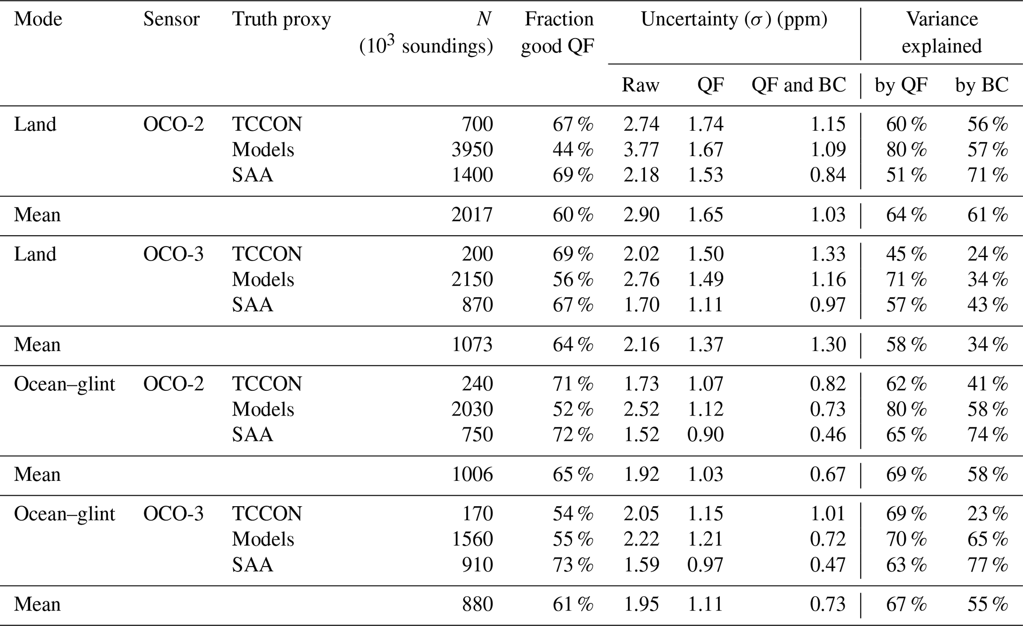
Table 7 provides a statistical summary of the results from the quality filtering and bias correction for both OCO-2 and OCO-3 for each of the three truth proxies. Results are given separately for land observations (combined nadir and glint) and for ocean–glint observations. The number of soundings contained in each truth proxy dataset that was used in the quality filtering and bias correction procedure is listed, along with the fraction of the total soundings contained in the L2 Lite XCO2 product that were assigned a good quality flag, i.e., the throughput. The standard deviation (σ) of the difference between the satellite XCO2 estimates and the truth proxy values is derived relative to (i) the raw XCO2 prior to bias correction, (ii) the quality-filtered XCO2, and (iii) the combined quality-filtered and bias-corrected XCO2. The two rightmost columns of the table show the percent of the variance explained by the quality filtering (compared to the raw XCO2) and the bias correction (compared to the quality filtered XCO2), respectively. The variance explained is calculated as , where σ1 is the original uncertainty (standard deviation) in the ΔXCO2 and σ2 is the remaining uncertainty. For each sensor and for both land and ocean–glint observations, the mean values from the three truth proxies are provided to help summarize the statistics.
Overall, the fraction of good-quality soundings remains the same at approximately 60 % for both sensors for land and ocean–glint. XCO2 estimates from both sensors exhibit comparable uncertainties in raw XCO2 against the three truth proxies of ≈ 2–3 ppm. Estimates from both sensors show a reduction in uncertainties after application of the quality filter first and then the combined quality filter and bias correction to approximately 1 ppm for land and 0.7 ppm for ocean–glint. Even though the mean of the uncertainties for the OCO-2 raw XCO2 versus truth proxies for land was higher (2.9 ppm) compared to OCO-3 (2.2 ppm), the mean of the uncertainties for the OCO-2 quality-filtered and bias-corrected XCO2 of 1.0 ppm is somewhat smaller than for OCO-3 at 1.3 ppm. This implies that the bias correction is more effective for OCO-2 than for OCO-3 over land. This is evidenced in the rightmost column of the table, which indicates that the OCO-2 bias correction explains 56 %–71 % of the variance (mean of 61 %) across the truth proxies, while only 24 %–43 % of the variance (mean of 34 %) is explained by the OCO-3 bias correction. For ocean–glint observations, the variance explained by the bias correction is similar for OCO-2 and OCO-3 at 58 % and 55 %, respectively.
The lower variance explained by the OCO-3 bias correction seems to originate from a combination of both a less effective dP correction and a much less effective CO2 grad del correction, a term related to the deviation in the retrieved CO2 profile from the prior. It is likely that the residual pointing errors in OCO-3 v10 of up to 1–2 km (median of ≈ 0.5 km), shown in Appendix B, produce a less accurate surface pressure prior, which in turn yields larger dP uncertainties from the L2FP retrieval. In addition, remaining radiometric calibration issues in the OCO-3 ABO2 spectral band may affect the retrieved surface pressure. Both of these factors could explain the less effective OCO-3 dP bias correction term. No viable explanation has yet been formulated for why the OCO-3 CO2 grad del bias correction term is so much less effective relative to that for OCO-2.
Improvements in successive versions of the ACOS L2FP retrieval are demonstrated in Fig. 1, which compares RMSEs in XCO2 from v9 and v10 OCO-2 as well as v10 OCO-3 versus the three truth proxies for land and ocean–glint observations. There are substantial decreases in the RMSE for OCO-2 from v9 to v10 compared to both TCCON and to the MMM for both land and ocean–glint. The changes in the OCO-2 RMSE from v9 to v10 for the small area analysis were insignificant between versions, which is to be expected because errors at very small spatial scales are primarily driven by instrument noise, which cannot be further reduced. For all three truth metrics versus land observations, OCO-3 compares worse than OCO-2. The discrepancy is likely driven by both OCO-3 residual pointing errors and L1b calibration errors, both of which are expected to improve in the next data version. The worse agreement of OCO-3 v10 with TCCON compared to OCO-2 v10 can be explained in part by the limited number of TCCON collocations with OCO-3 that were available at the time of creation of the QTS. Incidentally, the data also demonstrate that for all truth proxies and for both sensors, ocean–glint errors are lower than land errors, indicating higher precision relative to land observations. This result is at odds with previous findings showing unrealistic features in global inversion models which assimilate OCO-2 ocean–glint data (e.g., Peiro et al., 2022; Byrne et al., 2023).
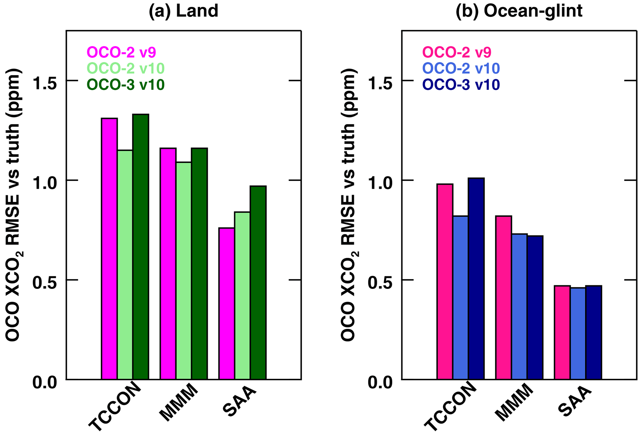
Figure 1RMSEs for different versions of OCO-2 and OCO-3 XCO2 versus three truth proxies: TCCON, multi-model median (MMM), and small area approximations (SAAs). Results are derived from single-sounding statistics using quality-filtered and bias-corrected XCO2 from the QTS. Results for land observations are shown in panel (a), while panel (b) shows results for ocean–glint observations.
Global maps showing the spatial distribution of the native sounding densities for a single year (2020) and a single footprint are shown in panels (a) and (c) of Fig. 2 for OCO-2 and OCO-3, respectively. The data here have been aggregated to 2.5∘ by 5∘ latitude–longitude grid cells, whereas the actual swath width of each sensor is on the order of 10 km. Although the total number of soundings collected is very similar (≈ 40 million), the distinct difference in latitudinal extent of the two sensors due to the orbital characteristics is evident. The polar orbit of OCO-2 provides nearly continuous latitudinal coverage. There is somewhat less coverage for orbit tracks over the northeastern Pacific because these orbits are used for data downlink, during which the OCO-2 instrument does not acquire science measurements. The precessing orbit of OCO-3 on the ISS limits coverage to latitudes less than ≈ 52∘, near which there is a high density of soundings at the orbit inflection points. In other words, OCO-3 produces a similar overall number of soundings compared to OCO-2, but the soundings are restricted to a smaller area, thus producing a higher density.
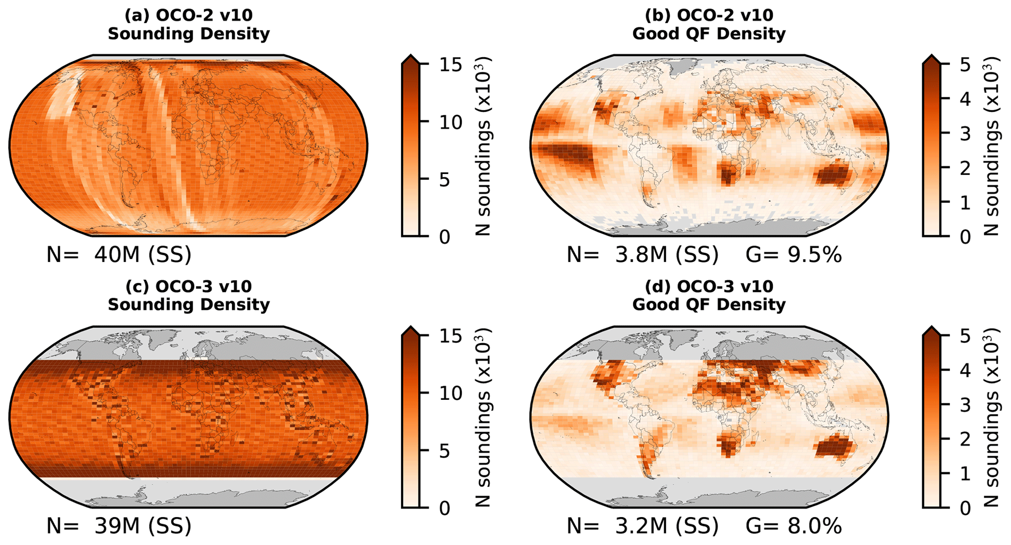
Figure 2Version 10 data volumes from a single detector footprint (4 of 8, 1-based) for the year 2020 gridded at 2.5∘ latitude by 5∘ longitude resolution for OCO-2 (a, b) and OCO-3 (c, d). The total number of measured soundings (N) for each sensor is shown in panels (a) and (c). Panels (b) and (d) show the number of soundings (N) that were assigned a good quality flag in the L2 Lite XCO2 product. The percent of the total number of measurements is given as G. Grid cells containing fewer than 10 soundings are colored gray.
The soundings that pass the preprocessor checks for cloud and aerosol loading and then converge in the L2FP algorithm are assigned either a good (QF = 0) or a bad (QF > 0) quality flag in post-processing. Typically, it is recommend that only the good-quality-flagged soundings be used in atmospheric inversion systems to deduce CO2 fluxes. Panels (b) and (d) of Fig. 2 show the sounding densities of the good-quality-flagged data for OCO-2 and OCO-3, respectively. Qualitatively, the distributions of good soundings from the two sensors resemble clear-sky fraction maps, as expected. Over land, OCO-3 provides more good soundings than OCO-2, especially near 50∘ latitude as a result of the ISS orbit. Furthermore, OCO-3 operates almost exclusively in nadir mode over land, which may also contribute to a higher good-quality sounding throughput relative to OCO-2 land–glint observations, which have higher optical path lengths and thus sensitivity to clouds and aerosols. Conversely, OCO-3 provides less good soundings over the oceans compared to OCO-2 due to lower sampling rates in glint observation mode as constrained by operations aboard the ISS. Mechanical and operational constraints on the OCO-3 instrument frequently preclude pointing towards the glint spot. During these periods, the instrument collects ocean data in nadir mode, for which the signal-to-noise ratio is too low to provide accurate estimates of XCO2.
Figure 3 shows bar plots quantifying the number of good soundings by month for each observation mode for the overlapping time period of August 2019 through February 2022 for OCO-2 (Fig. 3a) and OCO-3 (Fig. 3b). These plots help to visualize the difference in the ratio of land to ocean–glint observations for the two sensors. OCO-2 collects a much larger and more stable fraction of monthly ocean–glint compared to OCO-3. The lack of good-quality ocean–glint OCO-3 observations early in the mission is evident, as observations were often restricted to nadir-viewing mode due to safety concerns related to early uncertainties in the effects of polarization and signal levels for OCO-3, which were mitigated by revised PMA pointing with respect to the glint spot (Taylor et al., 2020). The plot also highlights the higher relative fraction of OCO-3 TG and SAM data (8 % of the total) compared to only 1 % TG data for OCO-2, a distinguishing characteristic that sets the two missions apart.
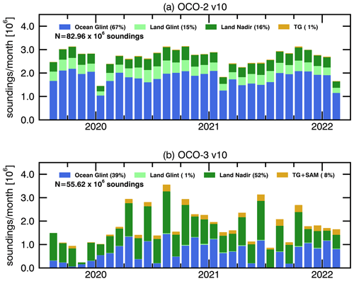
Figure 3Bar plots of the monthly number of good-quality-flagged soundings for OCO-2 (a) and OCO-3 (b) by observation mode (colors) for the time period of August 2019 through February 2022. The fractional percent for each observation mode is listed in the legend, along with the total number of good-quality-flagged soundings (N).
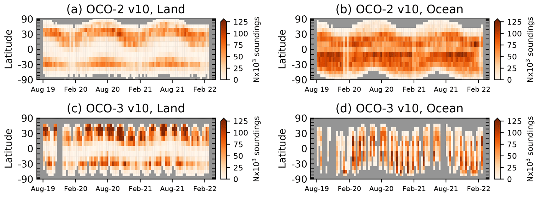
Figure 4Data density (103) of the number of good-quality-flagged soundings for v10 OCO-2 (a, b) and OCO-3 (c, d) for land (a, c) and ocean (b, d) at 10∘ latitude by 10 d resolution for the time period of August 2019 through February 2022. The ordinate axis is scaled by the cosine of the latitude to elucidate the decreasing fractional surface area of the Earth with increasing latitude. Grid cells containing fewer than 10 soundings are colored gray.
Figure 4 presents the densities of good data (QF = 0) gridded in time (10 d) and latitude (10∘) for OCO-2 (top) and OCO-3 (bottom). This again effectively demonstrates the difference in spatial coverage between the two sensors. The time–latitudinal coverage of OCO-2 is much smoother than OCO-3 due to the repeating sun-synchronous polar orbit. In contrast, OCO-3 has a sinusoidal-like pattern of alternating high and low densities over midlatitudes, with the maximum value alternating in time between the Northern and Southern Hemisphere. This is due to the precessing orbit of OCO-3 aboard the ISS, which introduces periodic variations in the portion of the Earth that is viewed during daylight hours. In addition, OCO-3 is subject to both predictable and unpredictable periods during which science measurements either cannot be collected at all or are limited to nadir viewing, as discussed in Appendix B. Predictable data gaps occur rather frequently for ocean–glint observations due to physical viewing constraints aboard the ISS JEM-EF. Periods of missing data that are longer than 10 d can be seen in Fig. 4d as columns that are fully gray.
As described in Sect. 1 of the OCO-3 v10.4 data quality statement (Chatterjee et al., 2022), early in the production of the OCO-3 v10 XCO2 Lite product, an analysis of XCO2 estimates collocated with OCO-2 soundings suggested that there was a diverging trend that was correlated with time since the last OCO-3 instrument decontamination cycle. After development and application of an “ad hoc” bias correction to the OCO-3 XCO2, the drift was eliminated, bringing the two sensors into agreement within the expected uncertainties of a few tenths of a part per million. A new set of OCO-3 L2 Lite XCO2 files (v10.4) was generated and distributed to the NASA Goddard Earth Sciences (GES) Data and Information Services Center (DISC) website (OCO Science Team et al., 2022). A full discussion of the ad hoc correction is provided in Appendix B. The remainder of the analysis that follows uses the OCO-3 v10.4 XCO2.
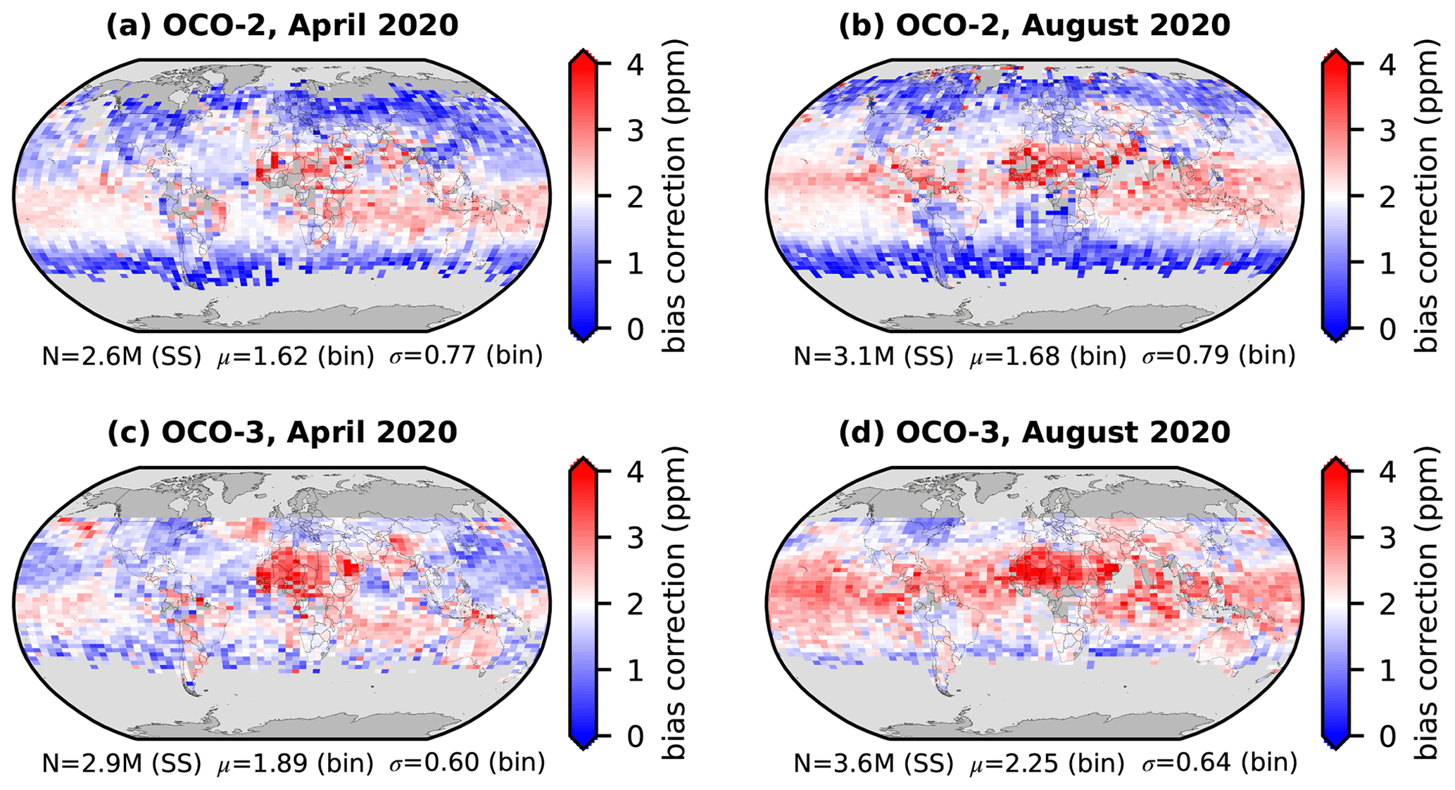
Figure 5Monthly maps of the bias correction for OCO-2 (a, b) and OCO-3 (c, d) for April 2020 (a, c) and August 2020 (b, d) gridded in 2.5∘ latitude by 5∘ longitude bins. The number of single soundings (SSs) is given by N, while the mean (μ) and standard deviation (σ) of the gridded (bin) data are reported. Grid cells with fewer than 10 soundings are colored gray.
Figure 5 shows maps of the magnitude of the bias correction (ppm) for both sensors for April and August 2020. The patterns look qualitatively similar, with bias corrections ranging from zero to ≈ 2 ppm in the midlatitudes and polar regions and bias corrections of up to ≈ 4 ppm over the Sahara and dust outflow regions, as well as the tropical oceans. The mean global bias corrections are slightly larger for OCO-3 compared to OCO-2 for both months, but the uncertainties are slightly smaller for OCO-3. The 2020 annual median bias correction was 1.81 ppm for OCO-2 and 2.11 ppm for OCO-3. Note that the OCO-3 v10.4 time-dependent ad hoc bias correction discussed in Appendix B3 has been removed.
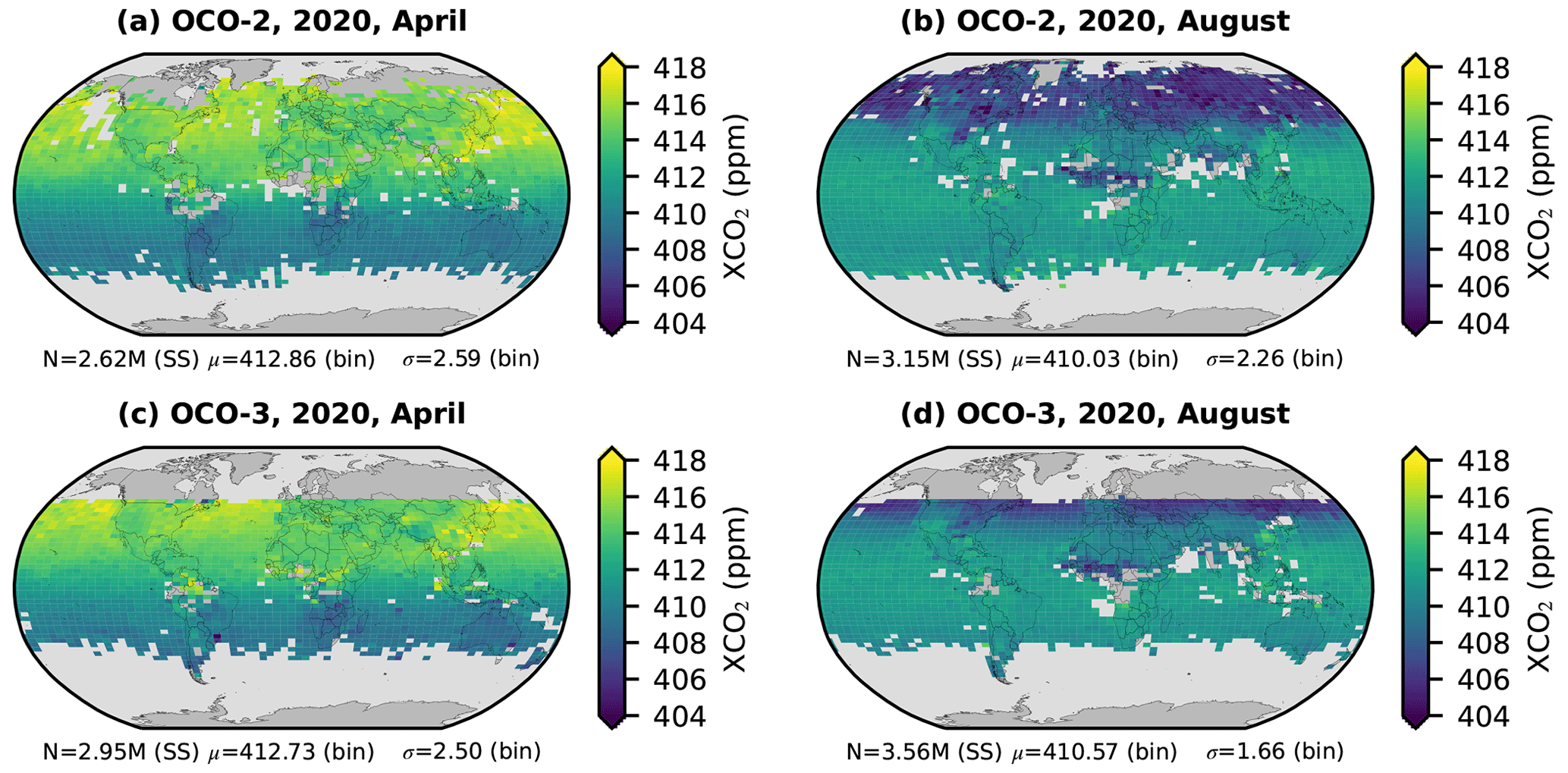
Figure 6Monthly maps of quality-filtered and bias-corrected XCO2 for OCO-2 (a, b) and OCO-3 (c, d) for April 2020 (a, c) and August 2020 (b, d) at 2.5∘ latitude by 5.0∘ longitude resolution. The number of single soundings (SSs) is given by N, while the mean (μ) and standard deviation (σ) of the gridded (bin) data are reported. Grid cells with fewer than 10 soundings are colored gray.
Figure 6 shows the spatial maps of OCO-2 and OCO-3 gridded quality-filtered and bias-corrected XCO2 for the months of April and August 2020. The well-known features of the atmospheric distribution of CO2 are present. For example, high values are observed in the Northern Hemisphere (NH) spring when the land biosphere is still quiescent (≈ 415 ppm), followed by lower values at high northern latitudes in August when the biosphere is most active (≈ 405 ppm). Since the seasonal cycle of CO2 is driven primarily by biospheric activity on land, the difference in April and August XCO2 in the Southern Hemisphere (SH) is much smaller compared to the NH. Although the distribution of XCO2 between the two sensors is qualitatively similar, the figures illustrate the difference in latitudinal coverage due to the differing orbit characteristics. This has meaningful consequences for the interpretation of flux estimates derived from inverse modeling of the OCO-2 and OCO-3 XCO2 concentrations. For example, OCO-3 cannot directly capture the strong summer drawdown of CO2 in the northern boreal forests. For this time and location, an inversion of OCO-3 CO2 fluxes must rely more on the model prior values since there is no information provided by satellite measurements, whereas an assimilation of OCO-2 XCO2 for this same time and location would provide information to the models since the satellite observed this location at this time. It is worth noting that it is challenging to produce a meaningful difference in XCO2 for the two sensors at the global scale due to the spatial and temporal differences in sampling. Generally, such maps look qualitatively like differences in CO2 driven by synoptic-scale weather patterns, as for any given grid box, there might be a difference of several days in observations from the two sensors. However, a direct comparison in XCO2 for a small set of collocated observations is provided in Appendix B3.
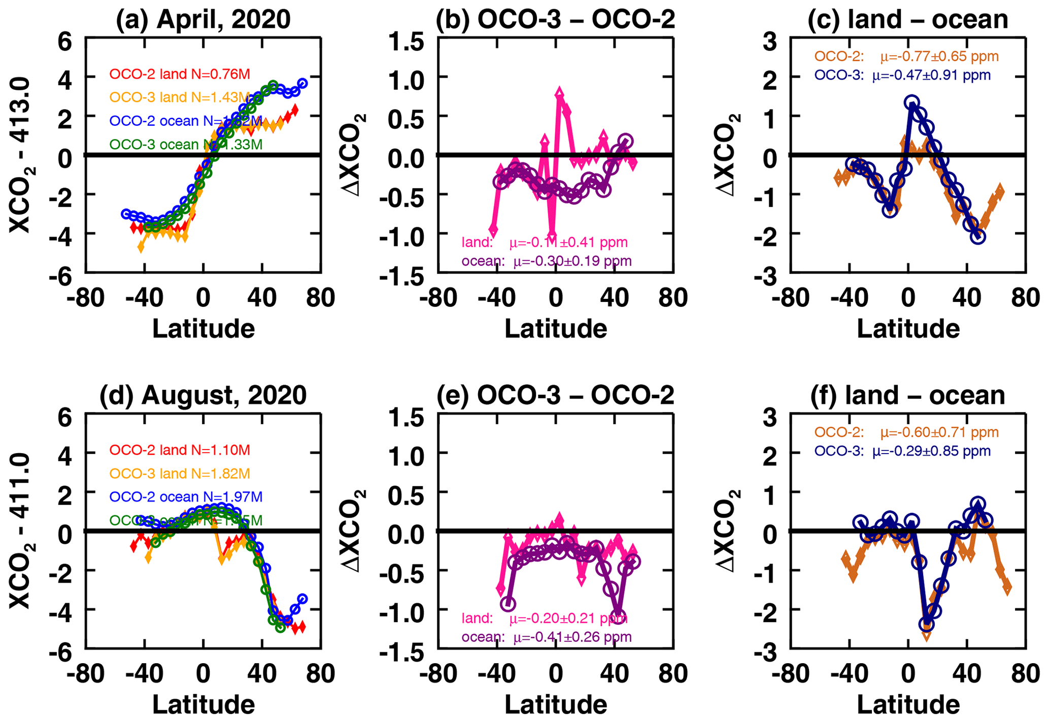
Figure 7Meridional XCO2 gradients at 5∘ latitude resolution by sensor and observation mode for April 2020 (a) and August 2020 (d). Only latitude bins containing at least 1000 soundings are shown. The total number of soundings (N) for each sensor and observation mode is given in the legend. Panels (b) and (e) show the differences in the monthly binned values (OCO-3 − OCO-2) for both land (pink diamonds) and ocean (purple circles) observations. Panels (c) and (f) show the differences in the monthly binned values (land − ocean) to demonstrate the land–ocean bias. The mean (μ) and standard deviation (σ) of the binned differences are given in the legend. Here, land observations include land–nadir, land–glint, land–TG, and land–SAM, while ocean includes ocean–glint observations.
To further demonstrate the agreement between the two sensors, panels (a) and (d) of Fig. 7 show the meridional behavior of XCO2 for both sensors and observation modes for April and August 2020, respectively. Here, the resolution is 5∘ latitude bins, and the monthly median OCO-2 XCO2 has been subtracted. In April, when XCO2 concentrations are near their annual maximums in the extratropical Northern Hemisphere, the meridional gradients are strong over both land and ocean. In August, when the Northern Hemisphere biosphere is fully active, XCO2 is within ≈ 1 ppm of the global median for latitudes below approximately 40∘ N but much lower than the global average at higher northern latitudes. The difference plots (OCO-3 − OCO-2), shown in panels (b) and (e) of Fig. 7, indicate that OCO-3 ocean–glint is generally biased low relative to OCO-2 by about 0.3 to 0.4 ppm with uncertainty, σ, of approximately 0.2 ppm. For land observations, the differences vary significantly with latitude, making inferences difficult. Panels (c) and (f) of Fig. 7 show the zonally averaged differences between land and ocean observations, which are expected to be close to zero for both sensors. Based on the results for these particular months, OCO-2 and OCO-3 are in approximate agreement, with land–ocean biases ranging ≈ ±2 ppm and significant variation by latitude. These same behaviors were observed for most months in 2020. This latitudinally dependent land–ocean bias is an unexpected feature of the dataset that requires further investigation. The analysis for April and August 2021 (not shown) was qualitatively very similar.
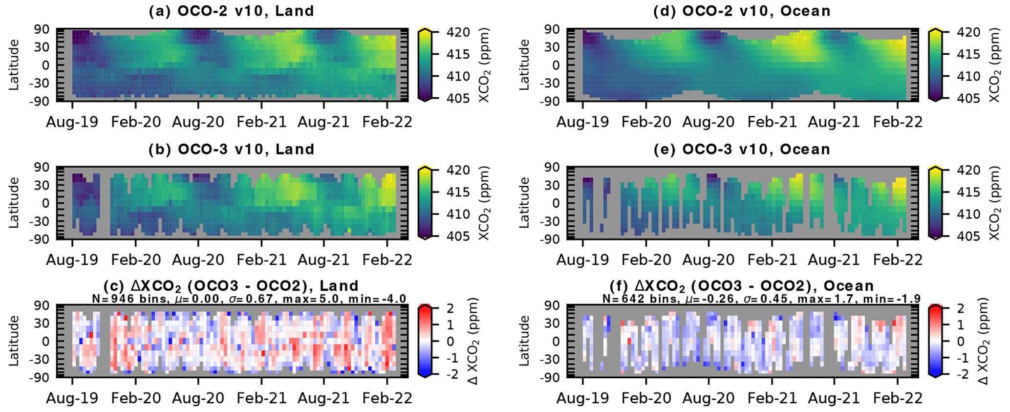
Figure 8Good-quality-flagged and bias-corrected XCO2 gridded at 10∘ latitude by 10 d for the overlapping time period of August 2019 through February 2022 for OCO-2 land (a) and OCO-3 land (b). The gridded differences for land observations (includes land–nadir, land–glint, land–TG, and land–SAM) are shown in panel (c). Panels (d), (e), (f) are the same, except for ocean–glint observations. The ordinate axis is scaled by the cosine of the latitude to elucidate the decreasing fractional surface area of the Earth with increasing latitude. Data cells with fewer than 10 soundings are colored gray. In panels (c) and (f) the number of valid grid cells (N) is given, along with the mean (μ), standard deviation (σ), and maximum (max) and minimum (min) differences in the gridded values.
Figure 8 shows XCO2 binned at 10 d by 10∘ latitude for the overlapping time period of August 2019 through February 2022 for OCO-2 (top row) and OCO-3 (middle row). Results are shown separately for land (left column) and ocean (right column). Qualitatively, the XCO2 patterns at this spatiotemporal resolution look very similar, as expected, with maximum XCO2 in NH spring just before the biospheric drawdown begins and minimums in NH summer. The plots highlight the secular trend of ≈ 2.2 ppm yr−1 and the seasonal variation in the latitudinal gradient of XCO2, which are both important features of the carbon cycle. Again, the substantial time periods during which no ocean data are collected by OCO-3 are evident in Fig. 8e.
Due to the vastly different sampling strategies of OCO-2 and OCO-3, coupled with spatial changes in XCO2 over short time periods, a direct comparison of observed XCO2 at a global scale is extremely difficult and can only be used to obtain a rough idea of how the sensors agree. Using the gridded values, the differences for land observations (Fig. 8c) have a mean value of 0.0 ppm, standard deviation of 0.67 ppm, and a range of +5 to −4 ppm. The ocean observations (Fig. 8f) exhibit a mean bias of −0.26 ppm (OCO-3 lower than OCO-2), with significantly lower uncertainty (0.45 ppm) and min–max (−1.9 and +1.7 ppm) compared to land. A more direct and accurate comparison between the two sensors, reported for a small subset of observations with tight spatial and temporal collocation, is discussed in Appendix B3.
This section discusses the evaluation of the OCO v10 good-quality-flagged XCO2 estimates against the truth proxies used in the quality filtering and bias correction procedure. Although there is some circularity in evaluating the satellite data against the same truth proxies used for filtering and bias correction, the multiparameter parametric bias correction is general enough so as not to overfit the OCO data. Furthermore, the truth proxies used for evaluation have been extended in time compared to the datasets used to train the filtering and bias correction. Although it is outside the scope of the current work, OCO-2 data have been validated against a range of other datasets, including in situ, NOAA and Aircore vertical observations (Rastogi et al., 2021), aircraft campaigns, e.g., ATom (Kulawik et al., 2019) and ACT-America (Bell et al., 2020), shipborne and airborne measurements (Müller et al., 2021), and EM27/SUN measurements (Jacobs et al., 2020).
6.1 OCO v10 XCO2 estimates versus TCCON
Section 3.3.1 introduced and discussed the TCCON data as used in the OCO v10 quality filtering and bias correction. Both OCO-2 and OCO-3 were quality-filtered and bias-corrected against TCCON GGG2014 data, while here TCCON GGG2020 XCO2 estimates are used in the comparison. Key changes to the retrieval algorithm between GGG2014 and GGG2020 are available on the TCCON wiki page (TCCON, 2023). The OCO quality filtering and bias corrections were trained using data through December 2018 for OCO-2 and December 2020 for OCO-3, whereas the validation data extend through February 2022 for OCO-2 and August 2022 for OCO-3. This provides some degree of independence in the evaluation.
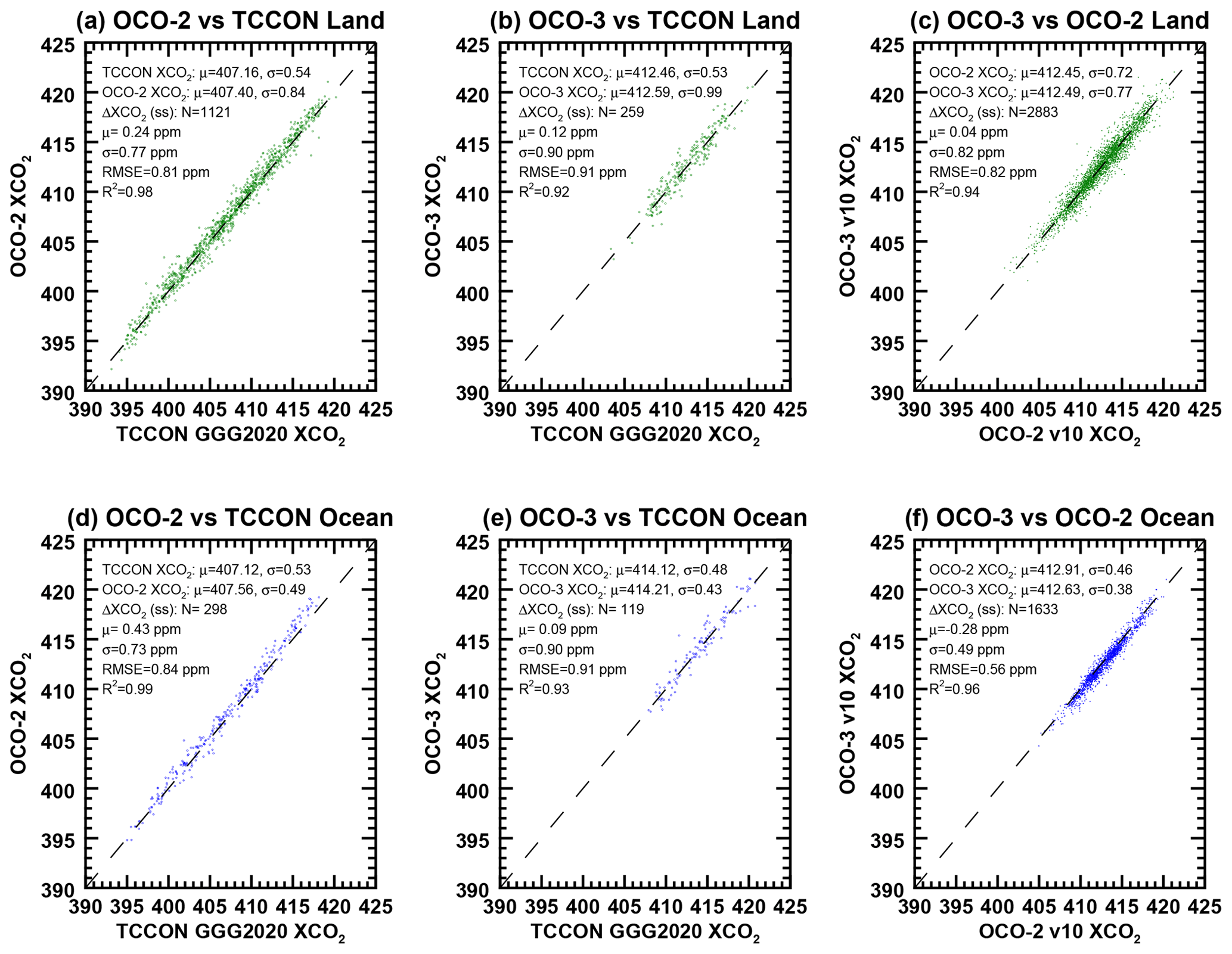
Figure 9One-to-one XCO2 correlation plots for land (a–c) and ocean (d–f) observations. Panels (a) and (d) show OCO-2 v10 versus collocated TCCON GGG2020 estimates, while panels (b) and (e) show OCO-3 v10 versus TCCON. Panels (c) and (f) show the correlation in OCO-3 versus OCO-2 XCO2, respectively, for the set of collocated soundings described in Appendix B3. In each panel, the top two rows of statistics give the mean (μ) of the XCO2 from all of the collocations and the mean standard deviation in the XCO2 (σ) from all of the collocations. The third through seventh rows of statistics give the number of collocations (N), the mean ΔXCO2, the standard deviation of the ΔXCO2, the RMSE (), and the coefficient of determination (R2: the squared Pearson linear correlation coefficient).
Figure 9 shows one-to-one correlation plots of the OCO-2 and OCO-3 v10 XCO2 estimates versus TCCON GGG2020 estimates, as well as the direct correlation between OCO-2 and OCO-3 using the collocated soundings that are presented in Appendix B. Each point on the graphs represents, for OCO, the mean XCO2 of the individual soundings acquired on a single overpass within a box 2.5∘ latitude by 5.0∘ longitude around a TCCON station. Only overpasses with at least 100 good-quality-flagged OCO soundings within the 2.5∘ latitude by 5.0∘ longitude grid box were retained. The TCCON values are the median of the XCO2 acquired within ±1 h of the OCO overpass.
For the 1121 OCO-2 land collocations (includes land–nadir, land–glint, and land–target) shown in Fig. 9a and the 259 OCO-3 land collocations (includes land–nadir and land–target) shown in Fig. 9b, the mean biases versus TCCON are 0.24 and 0.12 ppm, respectively, while the uncertainties are 0.77 and 0.90 ppm, respectively. In comparison, the OCO-3 vs. OCO-2 results, using the satellite collocations described in Appendix B, show a mean bias of 0.04 ppm with uncertainty of 0.82 ppm for land (Fig. 9c). This suggests that OCO-2 and OCO-3 agree with each other about as well as they agree with TCCON for land observations.
For the ocean–glint observations, OCO-2 exhibits a relatively high bias against TCCON of 0.43 ppm, with uncertainty of 0.73 ppm (Fig. 9d), while for OCO-3, the bias is 0.09 ppm with uncertainty of 0.90 ppm (Fig. 9e). It is important to note, however, that several of the TCCON stations that provide the bulk of the ocean–glint collocations had not yet processed their measurements through the GGG2020 version of the algorithm to provide estimates of XCO2. These stations include Ascension Island, Darwin, and Wollongong. When those data are available, more robust statistics will be calculated. Comparison of the OCO-2/3 ocean–glint collocations in Fig. 9f indicates that the bias between OCO-3 and OCO-2 ocean–glint is −0.28 ppm, with uncertainty of 0.49 ppm. This again suggests that the two sensors agree with each other in ocean–glint viewing approximately as well as they agree with TCCON.
6.2 OCO v10 XCO2 estimates versus models
To assess the impact of OCO XCO2 estimates on atmospheric inverse models, it is useful to compare the v10 product to results generated by an ensemble of carbon flux inverse models constrained by in situ measurements alone (e.g., O'Dell et al., 2018). This is done by calculating the difference between OCO retrievals from a reference XCO2 field; this difference is referred to as the “signal”. In the current work, the reference field is computed as the median of posterior concentrations from multiple models constrained by in situ measurements and is hereafter referred to as the multi-model median (MMM). The MMM provides a reasonable representation of XCO2 with seasonality and trends consistent with information derived from in situ measurements of atmospheric CO2 and does not necessarily represent the actual atmosphere at all spatiotemporal scales. This technique for looking at differences between satellite retrievals and modeled fields over broad, zonal regions is not new and has been employed in the literature for sanity checks (e.g., Chahine et al., 2008; Buchwitz et al., 2017; Zhang et al., 2017).
One of the contributions of satellite XCO2 estimates, such as those from OCO-2 and OCO-3, towards improving atmospheric flux inversion estimates is their ability to increase the density of global observations. A well-calibrated and precise satellite data record should offer the potential to reduce some of the uncertainties in the flux estimation associated with sparse sampling.
However, the global atmospheric transport models used in current-generation inversion studies have spatial resolutions of the order of 2 to 6∘ latitude and longitude. Such models cannot provide information with variability finer than several hundred kilometers. Rather than ingesting each individual OCO-2 XCO2 estimate falling inside a model grid box, down-sampling of the data into 10 s averages (10-sec-avg) prior to assimilation into inversion systems has become common (Crowell et al., 2019; Peiro et al., 2022; Byrne et al., 2023). This provides an even more compact dataset with reduced random sounding-to-sounding errors in the XCO2 estimates and mitigates the potential impact of correlated errors on ≈ 10 km spatial scales, such as those driven by surface features or the presence of aerosols and clouds (Massie et al., 2021; Mauceri et al., 2023; Massie et al., 2023). Care is taken to specify an appropriate measurement uncertainty, calculated as a function of the number of soundings within the 10-sec-avg bin, individual uncertainties associated with the soundings, coverage across the grid box, and correlations between their individual errors (Baker et al., 2022). In this study, XCO2 from the 10-sec-avg files is used to compare against the relatively spatially coarse model fields.
The models chosen for evaluation of the OCO v10 signal, identified in Sect. 3.3 and Table 6, all fit the following criteria: (i) each is constrained only by in situ measurements of CO2 concentrations in the atmosphere, (ii) each has been evaluated and vetted against independent data in the peer-reviewed literature, (iii) the simulated CO2 fields and surface fluxes are publicly available, and (iv) each simulation uses different atmospheric transport models and a unique inverse modeling framework (Table 5), thus sampling the full range of uncertainties in our present-day state-of-the-art knowledge of the atmospheric CO2 field.
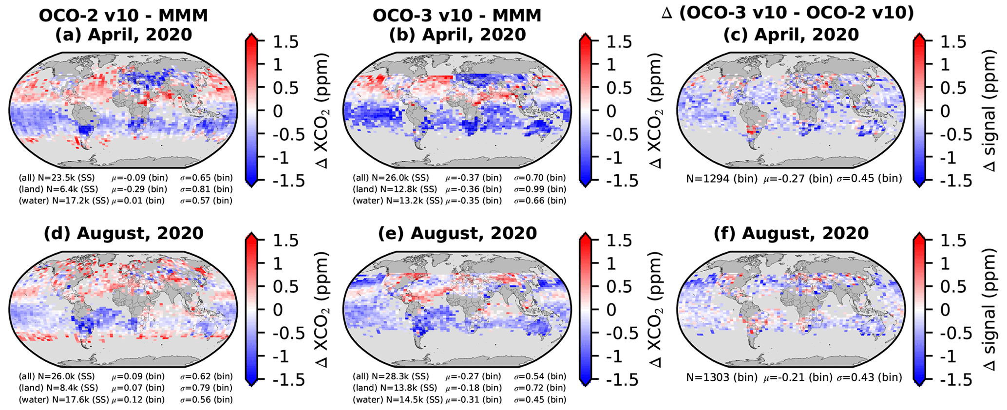
Figure 10Maps of XCO2 signal (XCO − XCO) at 2.5∘ latitude by 5∘ longitude resolution for April 2020 (a–c) and August 2020 (d–f) for OCO-2 (a, d) and OCO-3 (b, e). The numbers of single soundings (N SS) for all observation modes combined (all), combined land–nadir, land–glint, land–TG, and land–SAM (land), and water–glint (water) are given. The mean (μ) and standard deviation (σ) of the binned values (bin) are also given for each observation mode. Grid cells containing fewer than five soundings are colored gray. Panels (c) and (f) show the Δsignal (OCO-3 − OCO-2) for grid cells in which both sensors have valid data. Here, the statistics are given only for all observation modes combined.
Figure 10 shows maps of the signal at 2.5∘ by 5∘ lat–long resolution for April (top row) and August (bottom row) 2020 for OCO-2 (right column) and OCO-3 (middle column). Both sensors exhibit spatially coherent biases against models on the order of half of a part per million. Over oceans, the satellite estimates of XCO2 are generally biased low relative to the models in the SH and biased high in the NH. However, in the OCO-2 data, which extend further poleward compared to OCO-3, the high bias seems to occur at higher latitudes, both north and south. Following expectations, the uncertainty in the gridded data for both sensors in both months is higher for land (≈ 1 ppm) due to biases associated with topographic and surface albedo variability than it is for ocean (≈ 0.5 ppm), where these effects are minimal.
The differences in the gridded sensor signals are shown in Fig. 10c for April and Fig. 10f for August. Mathematically, the calculation is expressed as Δsignal = signalOCO-3 − signalOCO-2. Since the satellites sample the models at different times for individual soundings within a grid box, this calculation is not equivalent to a direct difference in the XCO2 between the sensors. Rather, it quantifies how different the satellite signals are from the MMM. The Δsignal values demonstrate that the two sensors agree better with each other than they do with the model suite in the region of overlap, as seen by the reduction in uncertainty to ≈ 0.45 ppm, with mean biases around 0.25 ppm in both months. Generally, OCO-3 is biased slightly higher against the MMM over land compared to OCO-2, while over ocean, OCO-3 is biased low against the MMM compared to OCO-2.
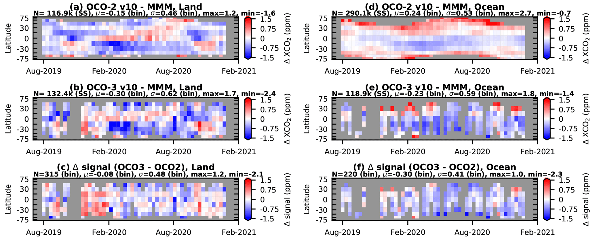
Figure 11The XCO2 signal (XCO − XCO) gridded at 10∘ latitude by 10 d for the time period of August 2019 through December 2020 for OCO-2 land (a) and OCO-3 land (b). The Δsignal for land observations (includes land–nadir, land–glint, land–TG, and land–SAM) is shown in panel (c). Panels (d), (e), and (f) are the same, except for ocean–glint observations. The ordinate axis is scaled by the cosine of the latitude to elucidate the decreasing fractional surface area of the Earth with increasing latitude. Data cells with fewer than 10 soundings are colored gray. In panels (a), (b), (d), and (e) the number of single soundings (N SS) is given, along with the mean (μ), standard deviation (σ), and maximum (max) and minimum (min) values of the gridded (bin) values. In panels (c) and (f) the number of valid grid cells (N) is given, along with the mean (μ), standard deviation (σ), and maximum (max) and minimum (min) differences in Δsignal.
A useful way to investigate the characteristics of the signal is by binning values into zonal (10∘ latitude) and 10 d bands, as seen in Fig. 11. Here, land observations, which include land–nadir, land–glint, land–TG, and land–SAM, are shown in the left column and ocean–glint observations on the right, with OCO-2 on the top row and OCO-3 in the middle. The model suite runs only through December 2020, so the graphs cover a 16-month period starting in August 2019. While the zonal mean tends to de-emphasize certain spatial features visible in the global maps, it brings out the temporal variations in the signal. Based on these results, coherent seasonal and latitudinal patterns in the signal are observed for both sensors. For land observations, both sensors tend to have positive signals in the NH and negative signals in the SH, while for ocean–glint observations, the signals tend to be positive poleward of the tropics in both hemispheres and negative in the tropics. The statistics calculated for the gridded signal data indicate that OCO-3 has higher uncertainty than OCO-2 (0.62 ppm vs. 0.46 ppm) and a larger bias (−0.30 ppm vs. −0.15 ppm) than OCO-2 for land observations, as seen in Fig. 11a and b. The statistics for ocean–glint signals indicate similar uncertainties between the two sensors of 0.53 and 0.59 ppm for OCO-2 and OCO-3, respectively, with mean biases of 0.24 and −0.23 ppm, as seen in Fig. 11d and e. The lower two panels of Fig. 11 show the differences in the gridded values (Δsignal) between the two sensors for land observations in Fig. 11c and for ocean–glint observations in Fig. 11f. The gridded mean difference between the two sensors for land observations is −0.08 ppm. The largest differences for land occur in December 2019, immediately following the OCO-3 PMA calibration that was described in Sect. 2.1.2 of Taylor et al. (2020), continuing through January 2020 when the next OCO-3 decontamination cycle occurred. The origin of this feature in the OCO-3 v10.4 XCO2 record is not currently understood. The gridded differences for ocean–glint observations, shown in Fig. 11f, indicate a mean low bias of −0.3 ppm for OCO-3 relative to OCO-2. Overall, as demonstrated with the maps in Fig. 10, these plots suggest that the two sensors tend to agree better with one another than they do with the model suite.
6.3 OCO v10 XCO2 estimates over small areas
Small areas, as introduced in Sect. 3.3.1, were used as XCO2 truth proxies in the development of the v10 quality filtering and bias correction. Small areas can also be used to derive realistic estimates of XCO2 uncertainties for assimilation into inversion systems (Baker et al., 2022; Peiro et al., 2022). For each small area, the “theoretical” uncertainty is calculated as the median value of the XCO2 uncertainties, which are described in Appendix B of O'Dell et al. (2012) and recorded in the L2Lite files. The “actual” uncertainty is calculated as the standard deviation of the retrieved XCO2 in each small area. A minimum of 40 OCO soundings are required for each small area. Ideally, the actual uncertainties are highly correlated with the theoretical uncertainties, with the relationship having a one-to-one dependence (slope, m = 1) and the y intercept falling at zero (y = 0). Figures 12 and 13 show the results of an analysis of the small area XCO2 uncertainties for land–nadir and ocean–glint observations, respectively.
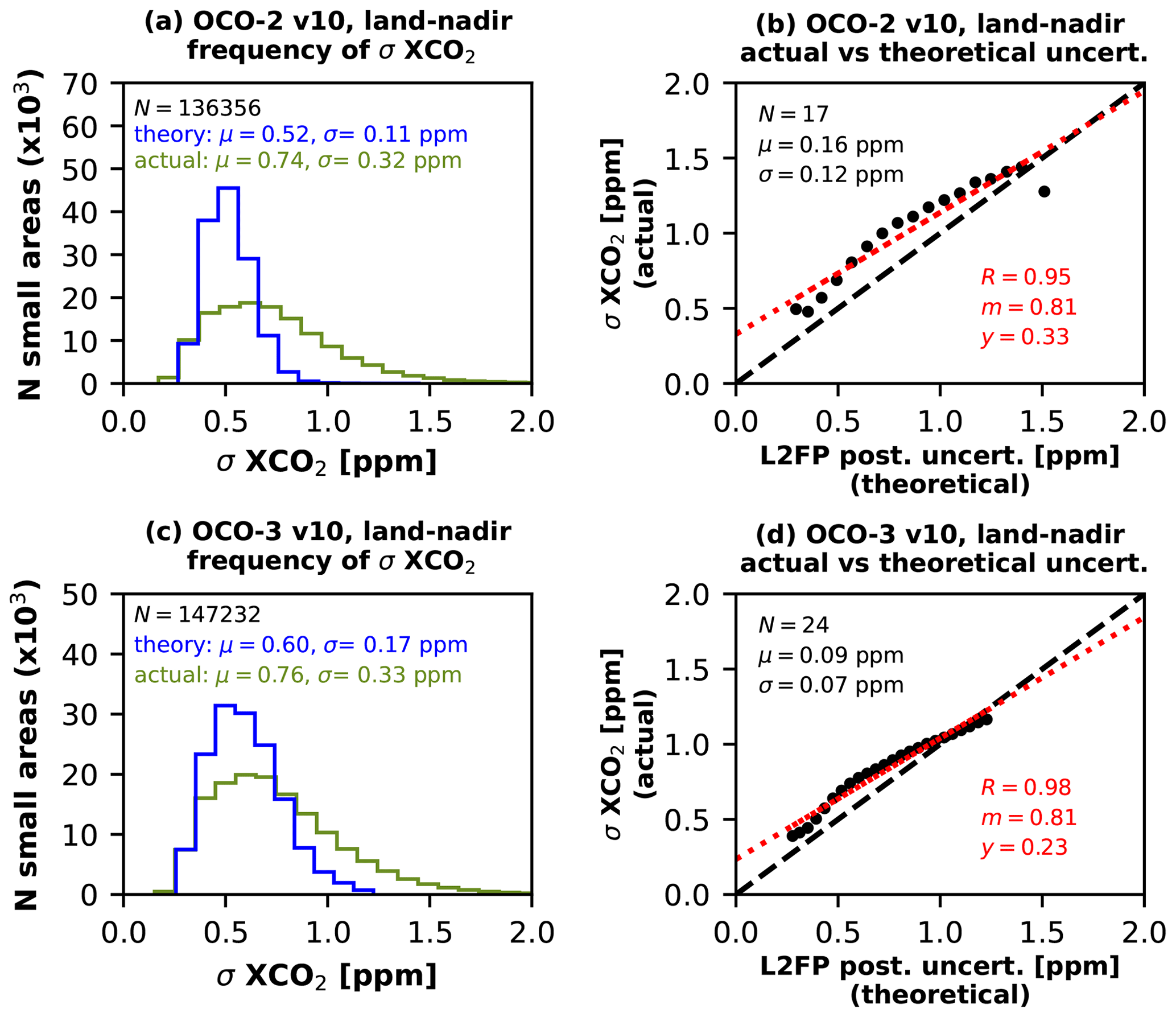
Figure 12Analysis of XCO2 uncertainties for land–nadir small areas for OCO-2 (a, b) and OCO-3 (c, d). Panels (a) and (c) provide the frequency distributions of both the theoretical uncertainties (blue curves) of the retrieved XCO2 as reported in the L2Lite file product (variable xco2_uncertainty) and the actual uncertainties (green curves) calculated from the standard deviation in the XCO2 for individual small areas. The number of small areas (N) as well as the mean (μ) and standard deviation (σ) of the theoretical and actual uncertainties are given in the legend. Panels (b) and (d) show the correlation of the actual uncertainties against the theoretical uncertainties using binned median values (black filled circles) to highlight deviations from the 1-to-1 line (dashed black line). A least-squares linear fit to the binned data is shown (dotted red line), along with the correlation coefficient (R), the slope of the fit (m), and the fit offset (y).
The frequency distributions of the XCO2 uncertainties over land–nadir small areas, as shown in panels (a) and (c) of Fig. 12 for OCO-2 and OCO-3, respectively, indicate that the actual uncertainties (green curves) are slightly larger with a wider distribution of values compared to the L2FP noise-driven theoretical uncertainties (blue curves). Although the actual uncertainties tend to be biased high, they are highly correlated with the theoretical uncertainties, having R values of 0.95 and 0.98 for OCO-2 and OCO-3, respectively, as seen in panels (b) and (d) of Fig. 12 for OCO-2 and OCO-3, respectively. Here, the median binned values are shown, rather than the uncertainties for individual small areas, to highlight deviations from the expected 1-to-1 relationship. These results imply that there are additional spatially correlated systematic uncertainties in the ACOS retrieval over small areas, and these additional uncertainties are similar for both sensors.
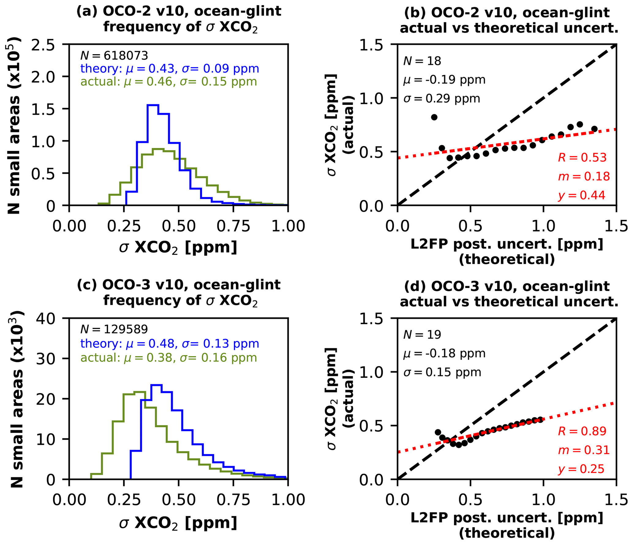
For ocean–glint observations, shown in Fig. 13, XCO2 uncertainties in small areas have different characteristics compared to land observations. The frequency distributions of the XCO2 uncertainties, shown in panels (a) and (c) of Fig. 13 for OCO-2 and OCO-3, respectively, indicate that the actual uncertainties (green curves) are often lower than the L2FP noise-driven theoretical uncertainties (blue curves), especially for OCO-3. Furthermore, even though the actual uncertainty correlates reasonably well with the theoretical uncertainty (R = 0.53 for OCO-2 and R = 0.89 for OCO-3), the line of best fit falls well off the expected one-to-one relationship, with a slope of 0.18 for OCO-2 and 0.31 for OCO-3. For the lowest theoretical uncertainties, the actual uncertainty is near or somewhat higher than anticipated, but when the theoretical uncertainties are large, the actual uncertainties are significantly lower than anticipated. This is unexpected for a well-characterized retrieval and indicates that there is some nonlinearity or other systematic behavior in the v10 ocean–glint retrieval. Early efforts to develop the OCO-2 v11 product suggest this is due to the parameterization of the ocean surface reflectance model. Additional investigation is underway.
6.4 OCO v10 XCO2 estimates along coastal crossings
Although not used in the parametric bias correction, the continuity of XCO2 estimates across coastlines (coastal crossings) provides a metric for detecting and correcting biases between land and ocean estimates of XCO2. Barring strong carbon sources or sinks, the true XCO2 should not change significantly at this transition, so the retrieved estimates should agree quite well. Here, a coastal crossing is defined as a set of contiguous soundings spanning approximately 50 km on either side of a land–water interface. The XCO2 values are quality-filtered and bias-corrected and include only glint-viewing-mode observations for both land and water. For OCO-2 v10, the coastal crossings were used, along with TCCON collocations and model fields, to determine the ocean–glint global scaling factor of 0.995, as described in Sect. 3.2.3 of the DUG (Osterman et al., 2020). For OCO-3 v10, the coastal crossings and model fields were used to determine the ocean–glint global scaling factor of 0.9961, as described in Sect. 5.1.5 of the DUG (Payne et al., 2022).
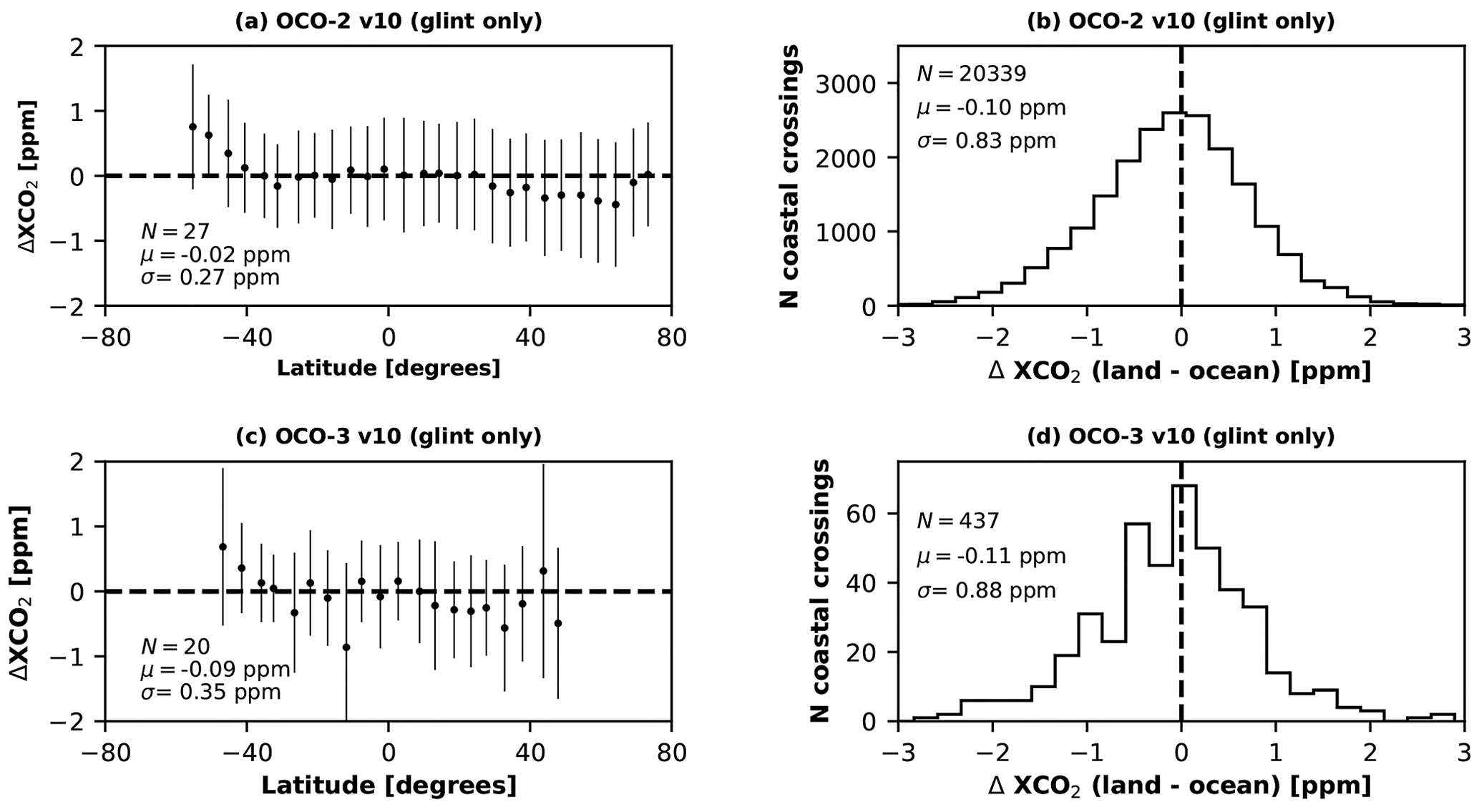
Figure 14Analysis of the coastal crossing dataset for OCO-2 v10 (a, b) and OCO-3 v10 (c, d). Panels (a) and (c) show ΔXCO2 (land–glint − ocean–glint) in 5∘ latitude bins with 1 standard deviation error bars as thin vertical lines. The number of latitude bins (N) and the mean (μ) and standard deviation (σ) of the binned values are given in the legend. Panels (b) and (d) show the frequency distributions of ΔXCO2 for the individual coastal crossings. The number of coastal crossings (N) and the mean (μ) and standard deviation (σ) of the XCO2 values for the individual crossings are given in the legend.
Figure 14 shows an analysis of the coastal crossing dataset for the v10 OCO-2 (top row) and OCO-3 (bottom row), containing ≈ 20×103 and 0.5×10³ crossings, respectively. Figure 14a and c show ΔXCO2 in 5∘ latitude bins with 1 standard deviation error bars as thin vertical lines. The mean land–ocean difference tends to be positive (negative) in the southern (northern) extratropical latitudes for both sensors. Figure 14b and d show the frequency distributions of ΔXCO2 for the individual coastal crossings. The means are biased −0.10 ± 0.83 and −0.11 ± 0.88 ppm for OCO-2 and OCO-3, respectively. The uncertainties are presumably due to local geometry, aerosol, and surface effects. In the future, an assessment should be made as to whether these biases can be explained by any retrieved parameters or other independent information such as population centers, which may help to shed light on the cause of these ubiquitous land–ocean XCO2 differences.
This work presents updates to the ACOS v10 retrieval algorithm used to derive estimates of XCO2 from the data collected by both the NASA OCO-2 and OCO-3 sensors. Four substantial changes were made to the L2FP code to provide better estimates of XCO2 relative to v9: (i) use of the ABSCO v5.1 absorption tables, (ii) calculation of more realistic prior aerosol information derived from daily GMAO GEOS-5 FP-IT model output, (iii) an update to the calculation of the CO2 vertical priors based on the GGG2020 algorithm, and (iv) implementation of a new solar continuum model based on TSIS-SIM measurements.
The quality filtering and bias correction implemented in the post-processing of the raw XCO2 estimates for v10 were briefly described. Overall, both the quality filtering and bias correction parameters selected from the training were similar to previous versions. It was shown that, while the efficacy of the quality filtering was similar for both sensors, the bias correction is more effective for OCO-2 than it is for OCO-3 for land observations. The remaining OCO-3 v10 pointing errors (median value of ≈ 0.5 km), coupled with residual instrument calibration errors, may introduce a less accurate surface pressure prior, which affects the efficacy of the dP bias correction term. The cause of a less effective CO2 grad del term in the OCO-3 v10 bias correction is still not understood.
Although the OCO-2 and OCO-3 sensors are similar, they provide different spatiotemporal coverage from their polar, sun-synchronous (OCO-2), and precessing (OCO-3) orbits. In particular, OCO-2 provides nearly full latitudinal coverage with a local sampling time of ≈ 13:36 ± 0.25 h, while OCO-3 is limited to latitudes ≈ ≤ 52∘ with variable local sampling time across a 63 d cycle. This work demonstrates, however, that the numbers of good-quality XCO2 estimates from the two sensors are approximately equal, albeit with different spatiotemporal coverage and quite different splits in observation modes. The OCO-3 sensor provides a larger fraction of good-quality soundings in nadir viewing over land, especially around 50∘ N latitude at the orbit inflection point. In addition, for OCO-3, nearly 10 % of its good-quality-flagged XCO2 estimates are taken in TG or SAM observation mode, allowing additional opportunities for targeting sites of interest, such as mega-cities and power plants (Wu et al., 2022; Roten et al., 2022; Lei et al., 2021; Nassar et al., 2022; Chevallier et al., 2022).
In this work, it has been demonstrated that the spatial and temporal distributions of XCO2 estimates from the OCO-2 and OCO-3 v10 products display the well-known features of the atmospheric distribution of CO2, including the Northern Hemisphere spring drawdown, the expected seasonal meridional gradients, and the secular trend of ≈ 2.2 ppm yr−1. After application of an ad hoc bias correction to the OCO-3 XCO2 by way of an L2 Lite file reprocessing to account for a time-dependent drift due to an L1b calibration artifact, the OCO-3 product agrees with OCO-2 within a few tenths of a part per million for a set of collocated soundings. This agreement is of a similar magnitude as the agreement of either sensor with the two truth proxies, TCCON and the multi-model median, for which RMSEs are on the order of 0.5 to 1 ppm. An analysis against small areas, which are contiguous regions smaller than 100 km over which the real uncertainty in XCO2 is expected to be less than ≈ 0.1 ppm, shows that the retrieval posterior uncertainties are underestimated by 20 %–40 % for land observations, while the uncorrelated relationship between actual and theoretical uncertainties for ocean–glint observations suggests deficiencies in the ACOS L2FP v10 ocean surface model. These deficiencies are expected to be mitigated in the next ACOS algorithm version. Additionally, a set of aggregated land–ocean XCO2 estimates from coastal crossings, used to deduce the global land and ocean scaling factors during the bias correction procedure, shows a global mean land–ocean difference of ≤ 0.1 ppm for both sensors, suggesting that the land–ocean bias has been mitigated.
As the science community continues work to better constrain the global carbon cycle (Crisp et al., 2022; Friedlingstein et al., 2022), top-down flux and inventory estimates utilizing XCO2 observations from space have demonstrated promise for answering key questions about the present and future response of the system to continued human activities and climate change (e.g., Byrne et al., 2021, 2022; Philip et al., 2022; Kong et al., 2022; Chevallier et al., 2022). The need for an international fleet of robust, dedicated carbon-monitoring satellites is paramount to this effort (Ciais et al., 2014; Crisp et al., 2018; Janssens-Maenhout et al., 2020; Palmer et al., 2022). The OCO-2 and OCO-3 records, which began in September 2014 and August 2019, respectively, will only gain in significance over time as an early baseline for globally monitoring CO2 concentrations from space. Overall, the results presented in this work indicate that a set of consistent estimates of XCO2 from OCO-2 and OCO-3, derived from a single retrieval algorithm (ACOS v10), compare well with one another. This suggests that the simultaneous assimilation of the two data records into atmospheric inversion systems has the potential to provide additional constraints on carbon fluxes relative to assimilating a single sensor.
While the discussion in Sections 4 and 5 focused on the 2.5-year overlap period with OCO-3, here, the full 7.5-year OCO-2 v10 data record is examined. The use of the OCO-2 v10 data record has already begun to appear in the published literature. Examples include an evaluation of the CO2 concentrations against the NOAA in situ network (Rastogi et al., 2021), quantification of power plant emissions (Nassar et al., 2021, 2022), detection of urban XCO2 gradients (Rißmann et al., 2022), a global and regional carbon budget analysis (Kong et al., 2022; Byrne et al., 2022), and an evaluation of global net carbon exchange based on a multi-model intercomparison project (Byrne et al., 2023).
Figure A1 shows a bar chart of the good-quality-flagged data volume for the full OCO-2 v10 data record, spanning 6 September 2014 through 28 February 2022. Here only one of the eight footprints per frame is represented. This figure highlights the stability in the data volume over the 7.5-year OCO-2 v10 record. During approximately the first year of operations, prior to the optimization of the scanning strategy implemented on 12 November 2015 as detailed in Sect. 5.2 of Crisp et al. (2017), the volume of good-quality-flagged data tended to be lower. Overall, the fractions of ocean–glint and land observations match those of the Earth proportions (≈ 70 % and 30 %, respectively). Due to the alternating nadir–glint viewing pattern, there is an even split between land–glint and land–nadir. The fraction of TG data is ≈ 1 % of the full science record. The most substantial instrument anomaly took place in August and September 2017 due to the temporary failure of the instrument baffle calibrator assembly door. However, regular planned decontamination cycles often interrupt OCO-2 science data acquisition for several days at a time.
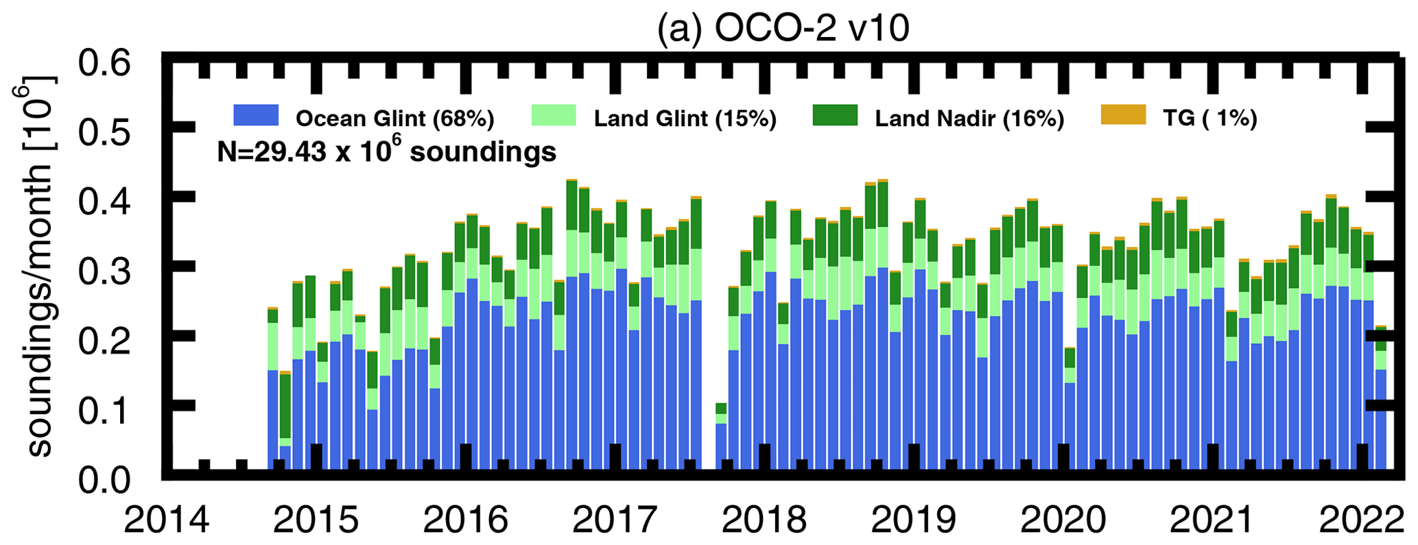
Figure A1Bar plots of the monthly number of good-quality-flagged soundings for a single footprint (4 of 8, 1-based) for the full OCO-2 v10 data record, spanning 6 September 2014 through 28 February 2022. Observation modes are distinguished by colors. The fractional percent for each observation mode is listed in the legend, along with the total number of soundings (N).
Figure A2 shows the OCO-2 v10 XCO2 binned by latitude (10∘) and time (10 d) from September 2014 through February 2022 for both land (Fig. A2a) and ocean (Fig. A2b). The dominant features of the atmospheric carbon cycle are observed, namely the secular increase of ≈ 2.2 ppm yr−1 (> 15 ppm over 7.5 years), the seasonal cycle with higher CO2 concentrations in the NH winter–spring, and lower values in the summer–autumn. In addition, the latitudinal dependence of the seasonal cycle is observed. The 7.5-year OCO-2 v10 XCO2 data record has the potential to allow for examinations of nearly decadal carbon cycle phenomena, as has been done with the 11.5-year GOSAT v9 record (Jiang et al., 2022).
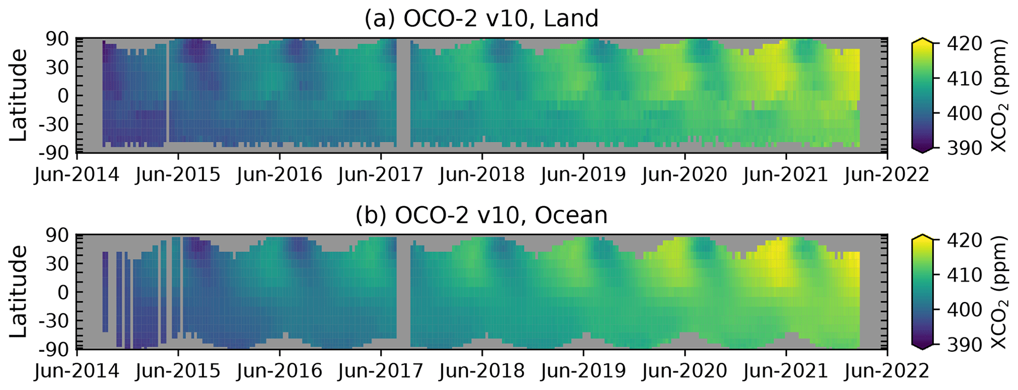
Figure A2OCO-2 v10 XCO2 gridded at 10∘ latitude by 10 d for the time period of September 2014 through February 2022. Panel (a) includes land–nadir, land–glint, land–TG, and land–SAM (Land) soundings, while panel (b) is for ocean–glint soundings. The ordinate axis is scaled by the cosine of the latitude to elucidate the decreasing fractional surface area of the Earth with increasing latitude. Grid cells containing fewer than 10 soundings are colored gray.
Figure A3 provides a brief analysis of the CO2 concentrations and atmospheric growth rates (AGRs) calculated from the OCO-2 v10 7-year record. This figure is a reproduction of Fig. 2 in Buchwitz et al. (2018). Shown in Fig. A3a are the globally averaged, monthly values of XCO2 for OCO-2 land observations (orange), along with the most recent ACOS GOSAT XCO2 (v9; Taylor et al., 2022) in gray, and the global monthly mean marine surface values reported by NOAA GML (Dlugokencky and Tans, 2022) in blue. Here, a cosine of latitude factor has been applied to the satellite data to weight individual soundings for surface area, i.e., higher (lower) weighting in the tropics (high latitudes). It is important to distinguish differences in the NOAA and satellite products. NOAA's values are calculated from precisely calibrated surface observations at a few select locations (Conway et al., 1994), while OCO-2 and GOSAT provide full column measurements with much larger random errors (instrument plus retrieval), as well as spatial and temporal sampling biases, but for hundreds to thousands of samples per day.
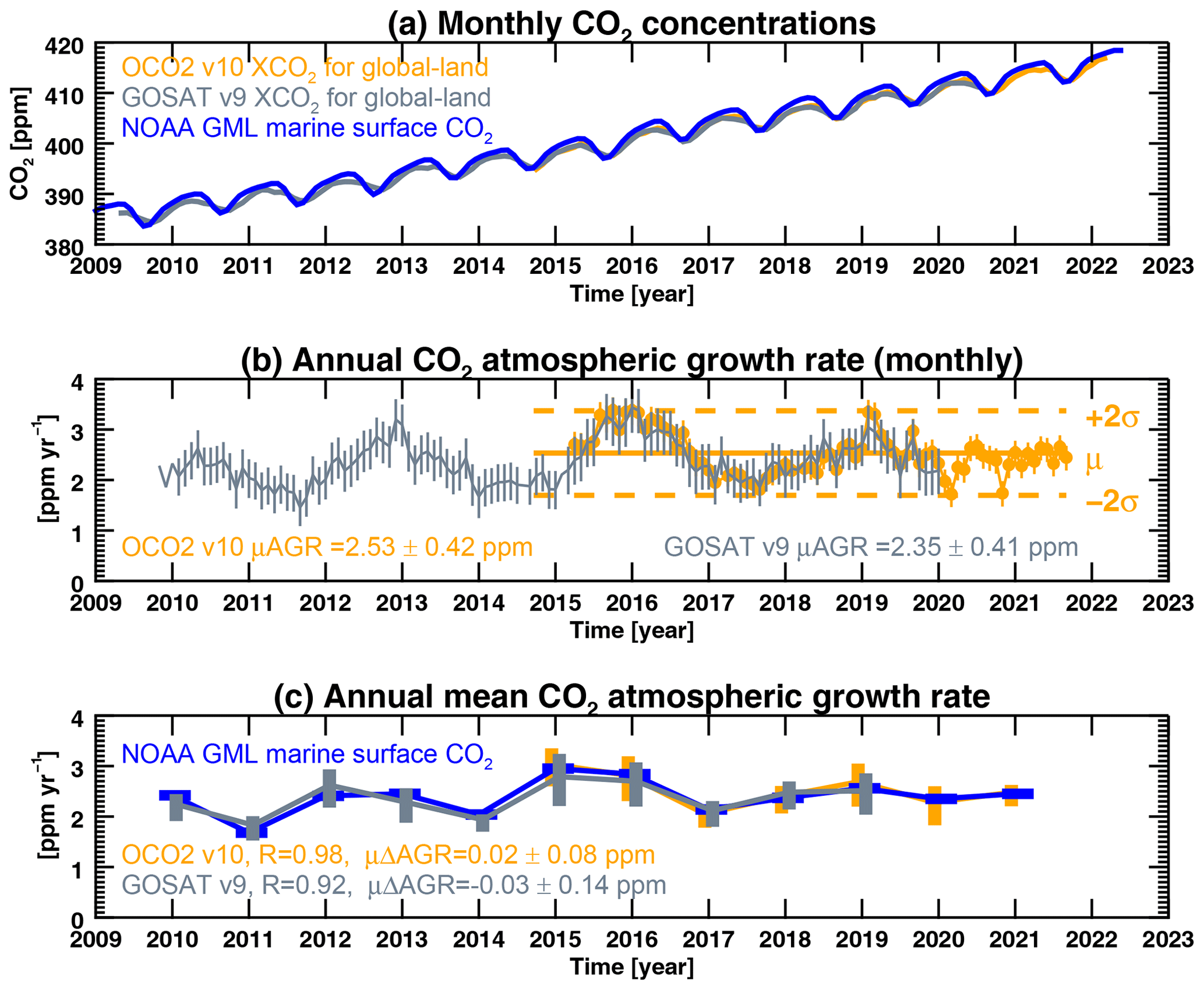
Figure A3CO2 concentrations and calculated atmospheric growth rates (AGRs) from the OCO-2 v10 data record (orange), with a comparison to ACOS GOSAT v9 (gray) and NOAA GML marine surface values (blue), similar to Fig. 2 in Buchwitz et al. (2018). Panel (a) shows the monthly CO2 concentrations for each product. Panel (b) shows the calculated monthly values of the AGR with vertical error bars (see text for description of how the error is calculated). The mean (μ) monthly AGR is indicated with corresponding standard deviation. Panel (c) shows the calculated annual AGRs. The linear Pearson correlation coefficient (R) of the satellite versus the NOAA GML values is given, along with the mean difference in the annual AGR (μΔAGR) with corresponding standard deviation.
Panel (b) of Fig. A3 shows the monthly calculated AGRs from the OCO-2 v10 (orange) and GOSAT v9 (gray) datasets. Here the vertical error bars are calculated as the mean of two individual error terms divided by the number of valid months within a given calendar year. The error terms are (i) the mean value of the XCO2 uncertainty for individual soundings within the month and (ii) the mean of the standard deviation of the calculated AGRs within the calendar year. The monthly average OCO-2 AGR over the 7.5-year record is 2.53 ± 0.42 ppm, shown here as a solid line. The dashed lines indicate the ±2σ level. The sharp increase in AGR during the middle of 2015 due to the strong El Niño is observed (Chatterjee et al., 2017; Liu et al., 2017), followed by a slow decreasing period from early 2016 to early 2017. The AGR was then stable through the end of 2018, when a second sharp increase was observed due to the weak 2019 El Niño. After some decline through early 2020, the AGR remained relatively constant through the end of the reported record (autumn 2021). The GOSAT v9 AGRs agree quite well with the OCO-2 v10 for the overlapping time period.
Panel (c) of Fig. A3 compares the annual growth rates of OCO-2 v10 and GOSAT v9 (the annual mean of the monthly values shown in Fig. A3b) to the NOAA GML annual marine surface values. The satellite AGRs generally agree to within a tenth of a part per million or less. The correlation coefficient across the 7-year OCO-2 record is 0.98 with a mean difference of 0.02 ± 0.08 ppm. The maximum difference of 0.13 ppm occurred in 2019, presumably due to the high AGR peak seen by OCO-2 in the first quarter.
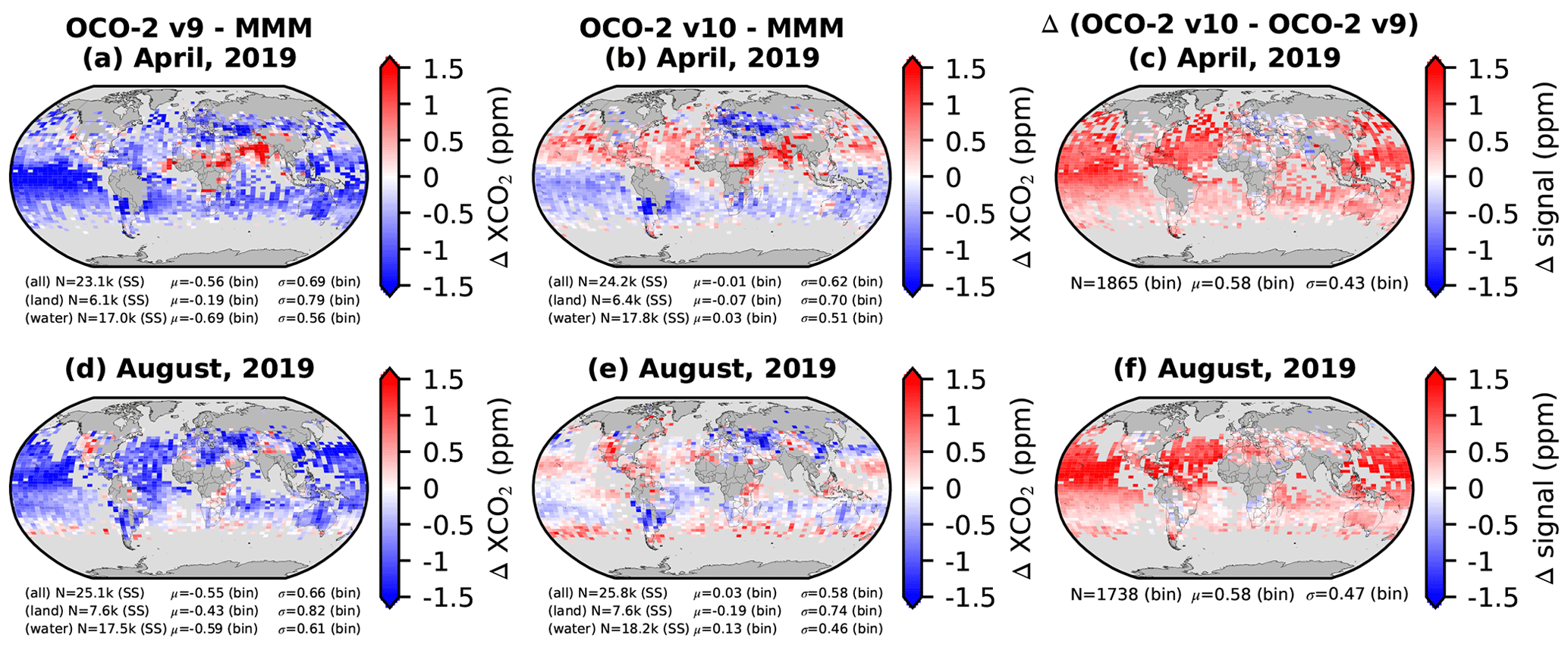
Figure A4Maps of XCO2 signal (XCO − XCO) at 2.5∘ latitude by 5∘ longitude resolution in April 2019 (a–c) and August 2019 (d–f) for OCO-2 v9 (a, d) and OCO-2 v10 (b, e). The numbers of single soundings (N SS) for all observation modes combined (all), combined land–nadir, land–glint, land–TG, and land–SAM (land), and water-glint (water) are given. The mean (μ) and standard deviation (σ) of the binned values (bin) are also given for each observation mode. Grid cells containing fewer than five soundings are colored gray. Panels (c) and (f) show the Δsignal (OCO-2 v10 − OCO-2 v9) for grid cells in which both sensors have valid data. Here, the statistics are given only for all observation modes combined.
To get a sense of the improvement in the OCO-2 v10 XCO2 product relative to v9, Fig. A4 shows maps of XCO2 signal (XCO − XCO) at 2.5∘ latitude by 5∘ longitude resolution for April (top row) and August (bottom row) 2019 for OCO-2 v9 (left) and OCO-2 v10 (middle). The right column shows the Δsignal (OCO-2 v10 − OCO-2 v9) for grid cells in which both v9 and v10 have valid data. Generally, for April and August 2019, the global bias against models is smaller for OCO-2 v10 (≤ 0.3 ppm) than it was for v9 (≥ 0.5 ppm), with a slight reduction in uncertainty from > 0.65 ppm to ≈ 0.60 ppm. The Δsignal values indicate that OCO-2 v10 XCO2 is shifted ≈ 0.6 ppm higher than v9. Most of the difference is in the ocean, whereas the changes in land XCO2 were relatively small between versions. Although the details vary, corresponding plots for other months and years (not shown) look similar.
B1 OCO-3 operations
As was discussed in Taylor et al. (2020), the collection of science data by OCO-3 is often interrupted by either the Hunstville Operations Support Center (HOSC) or the Mission Operations System (MOS) at JPL. Interruptions by the HOSC are generally due to arriving or departing vehicles from the ISS or other ISS activities such as spacewalks or instrument outgassing events. OCO-3 also suffers from data drop-outs in ocean–glint viewing due to physical obstructions within the field of view, e.g., solar panels.
Table B1Monthly statistics of the OCO-3 collection for the period of August 2019 through February 2022.
Table B1 shows the statistics at a per-granule (orbit) level for OCO-3 from August 2019 through February 2022. Over the course of these 31 months, HOSC interruptions occurred for ≈ 9 % (1329) of the total number of granules (14 527), while MOS interruptions occurred for ≈ 8 % (1038) of the observable granules (13 198), yielding 12 160 granules containing science measurements (≈ 92 % of the observable, 84 % of total). This well exceeds the mission requirement of 50 % data acquisition.
B2 OCO-3 v10 pointing correction
Although the first public release of OCO-3 XCO2 (vEarly) was derived using the v10 L2FP algorithm, the dataset suffered from significant geolocation errors (Taylor et al., 2020). Here, an update in the geolocation for v10 is described.
Precise geolocation of OCO-3 footprints requires knowledge of (i) the position and attitude of the instrument in space, (ii) the position and control of the PMA, and (iii) the effective alignment of the OCO-3 detectors with respect to the instrument reference. Improvements were made in all three areas for v10, as described in Sect. 2.2 of the OCO-3 v10.4 data quality statement (Chatterjee et al., 2022). OCO-3 attitude data are now taken primarily from the onboard stellar reference unit (SRU), which was not possible for vEarly due to a systems timing error that yielded large geolocation errors early in the mission. When the SRU is not available for attitude information, the OCO-3 processing stream relies on stellar reference data from the CALorimetric Electron Telescope (CALET) (Torii and Marrocchesi, 2019), another instrument aboard the ISS JEM-EF. During early operations, the PMA was calibrated using measurements from the onboard internal context camera (ICC), and an external lookup table was derived for azimuth and elevation angle offsets. For v10, a model fit to the PMA calibration data was implemented directly into the geolocation algorithm. Finally, for OCO-3 v10, the effective alignment of the detectors with the instrument reference was empirically determined using a best-fit static alignment adjustment. An additional rotation element was added to the geolocation algorithm, and the relative alignment space was systematically explored using a metric derived from minimizing surface pressure errors and albedo differences. This removed a systematic pointing error of 1 to 2 km. Overall, adjustments to the OCO-3 geolocation led to an improvement in the pointing errors from 1–2 km in vEarly down to typically less than 1 km in v10. Further refinements to OCO-3 geolocation are expected in future versions.
To confirm the v10 pointing errors, a pointing optimization code was developed to examine the residual errors for individual swaths within a collection of SAMs. The code minimizes a cost function using the difference in retrieved and modeled surface pressure (the L2FP prior), coupled with differences in the weak CO2 surface albedo between the retrieved values from the IDP and the black-sky albedo from MODIS Band 6, using the closest-in-time available MODIS albedo file (1 km resolution, product MCD43A3; Schaaf, 2022). The primary result of the code is an optimal shift in latitude and longitude for each swath in a given OCO-3 SAM or target observation to bring it into alignment with the ancillary data. Note that SAM swaths are not actually displaced by the suggested optimization values within the v10.4 data products, and thus geolocation errors typically up to 1 km remain in OCO-3 v10 data. However, for future reprocessing, a final optimization on all SAMs in the data collection prior to public release may be considered, depending on the residual errors. In specific instances, the project has supported requests to optimize individual SAMs in support of science analysis, as was done for Nassar et al. (2022).
Figure B1 shows analysis of the OCO-3 v10 pointing offset optimization results for a set of a few hundred SAMs collected over an approximately 1-year period. As each SAM consists of between four and six swaths, the total swath count is 372 after several quality assurance criteria are applied based on the certainty of the results for each fit. Figure B1a provides the frequency distribution of the optimization distance (Δ d) for vEarly (pink) and v10 (blue). While the mean median Δ d was ≈ 1.5 km in vEarly, for v10 the optimization distance has been reduced to ≈ 0.5 km.
Figure B1Comparison of OCO-3 pointing optimization for vEarly (pink) and v10 (blue) spanning an approximately 1-year time period. Panel (a) shows the frequency distribution of the optimization distance. The orbit ranges and number of swaths are indicated in the legend, along with the mean, median, and maximum optimization distances (dx) in kilometers. Panel (b) shows the cumulative frequency distributions. The percent of the swaths (Frac N) with optimization distances greater than 1.25, 2.5, and 5.0 km are indicated in the legend.
Panel (b) of Fig. B1 shows the cumulative frequency distribution, which indicates that for vEarly ≈ 65 % of the swaths had Δ d > 1.25 km, while for v10 the fraction of swaths with Δ d > 1.25 km has been reduced to ≈ 15 %. In the vEarly product, more than 7 % of the swaths had Δ d > 2.5 km, while for v10, less than 1 % of the swaths have a pointing error greater than 2.5 km. Recall that the nominal size of an OCO-3 footprint is 1.6 by 2.2 km. An additional reduction in the OCO-3 pointing error to the sub-0.5 km level, on order with OCO-2 (Kiel et al., 2019), is the nominal goal for a future reprocessing.
B3 OCO-3 v10 ad hoc XCO2 bias correction
The ad hoc correction to OCO-3 v10 XCO2 using collocated OCO-2 data is predicated upon the hypothesis that two sensors measuring the same column of air at the same time should produce the same XCO2 estimate when derived using the same retrieval algorithm. Therefore, a set of spatiotemporal collocations between the OCO-2 and OCO-3 sensors was identified over the time period of 6 August 2019 through 31 October 2021. If the XCO2 values from the two sensors are in good agreement, the expectation is for a mean bias close to zero, with low variability and no time trend.
Each OCO-2/3 collocation consists of a cluster of soundings for each of the two sensors measured within a 25 km radius and ±4 h time and containing at least 15 good-quality-flagged soundings per sensor. The difference in the mean bias-corrected XCO2 (μ) for each collocated cluster of soundings (ΔXCO2 = μ OCO-3 − μ OCO-2) provides a reasonably direct comparison between the sensors.
Figure B2XCO2 from simultaneous nadir overpasses (SNOs) between the OCO-2 and OCO-3 over eastern Europe on 12 August 2019 (A) and over the southwestern coast of Africa on 22 September 2021 (B). In example (A) the time difference between the overpasses was 282 s (< 5 m) and the difference in the average XCO2 from the two sensors was 0.17 ppm. In example (B), the time difference was 1519 s (25 m) and the difference in the average XCO2 from the two sensors was 0.01 ppm. The uncertainty in XCO2 for the entire scene was about 0.5 to 0.8 ppm for both sensors. The background for these image comes from ArcGIS, available at https://server.arcgisonline.com/ArcGIS/rest/services (last access: 1 May 2022). Note that the collocation criteria used in this work (25 km radius and ±4 h) mean that not all collocations were direct simultaneous overpasses, and a mixture of both nadir and glint viewing was used.
Figure B2 provides two example visualizations of overlapping orbit tracks from OCO-2 and OCO-3 as measured over eastern Europe on 12 August 2019 (A) and over the southwestern coast of Africa on 22 September 2021 (B). In example (A) the time difference between the overpasses was < 5 min, with a ΔXCO2 of 0.17 ppm. In example (B), the time difference was 25 min, with a ΔXCO2 of 0.01 ppm. The variability in XCO2 for the entire scene was about 0.5-0.8 ppm for both sensors.
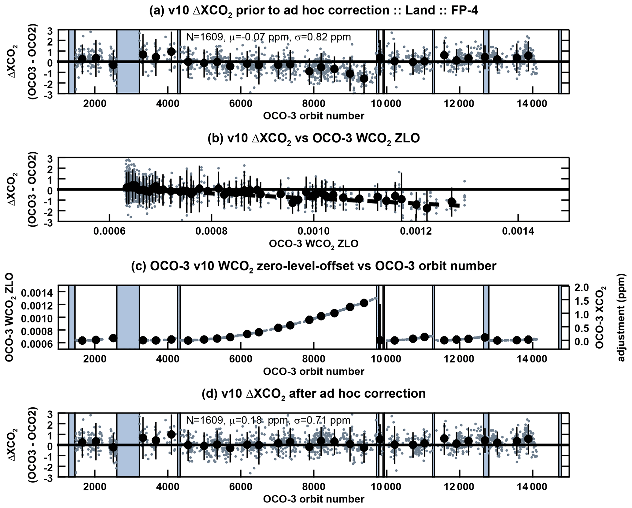
Figure B3Ad hoc bias correction of OCO-3 v10 XCO2 for footprint 4 (FP-4) land measurements. Panel (a) shows the ΔXCO2 (OCO-3 − OCO-2) for a set of collocated clusters of soundings versus the OCO-3 orbit number. The number of collocations (N) and the mean (μ) and standard deviation (σ) of the ΔXCO2 are given in the legend. Panel (b) shows the correlation between the ΔXCO2 and the OCO-3 WCO2 ZLO used to determine the correction. Panel (c) shows the OCO-3 WCO2 ZLO (left) and magnitude in parts per million (ppm) of the ad hoc XCO2 bias correction (right) versus OCO-3 orbit number. Panel (d) is similar to panel (a), except with the OCO-3 XCO2 ad hoc correction applied. In all panels, the small gray dots indicate individual collocations, while the large black dots are binned median values. The vertical shaded regions in panels (a), (c), and (d) indicate the time period during which the OCO-3 instrument was powered down for a decontamination cycle.
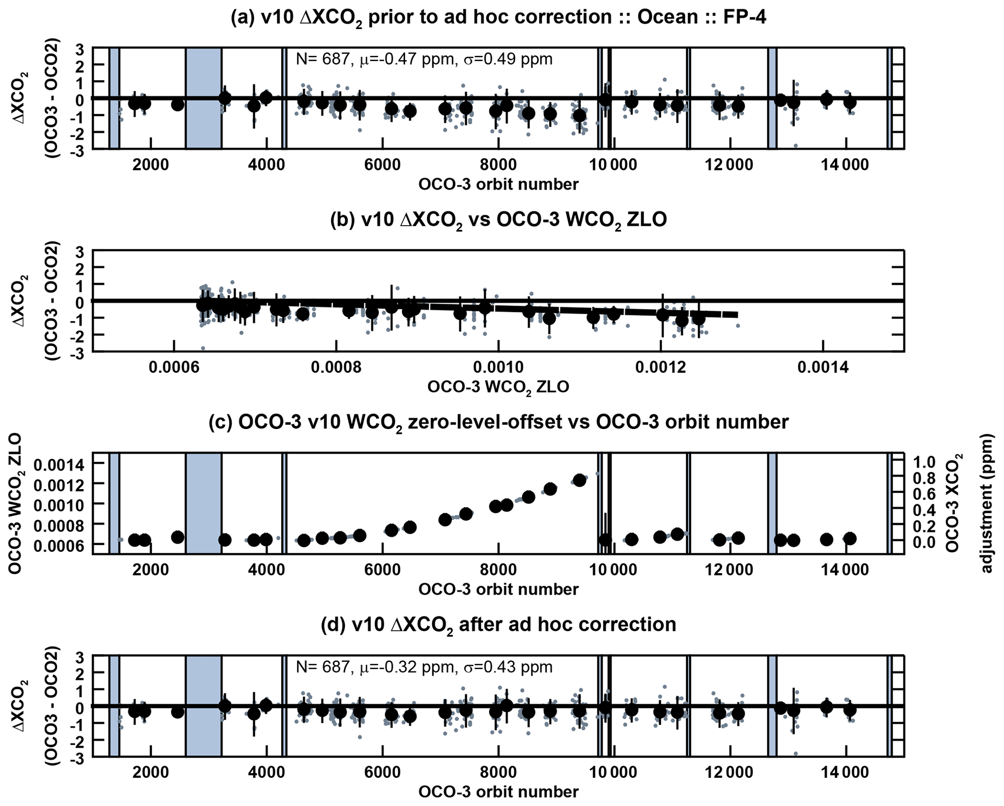
Time series plots of the ΔXCO2, as shown in panel (a) of Fig. B3 for land observations and panel (a) of Fig. B4 for ocean–glint observations, suggest a significant divergence in ΔXCO2 between orbits 4339 and 9719 (February 2020 through January 2021). This time period corresponds to a long interval with no instrument decontamination, which is indicated by the shaded areas in the plot. Upon investigation, it was found that the diverging ΔXCO2 correlates with an OCO-3 L1b calibration artifact: the instrument stray light, or zero-level offset (ZLO), as shown in Fig. B3b. The band-dependent ZLO is derived from measurements of the onboard calibration lamps on the unilluminated pixels of the detector and is found to increase nonlinearly in time since the last decontamination cycle, as shown against the left ordinate in Fig. B3c.
A correction to the OCO-3 XCO2 values (right ordinate of Fig. B3c) is derived from a linear fit of the ΔXCO2 (at a given orbit) versus the WCO2 ZLO at the same orbit (Fig. B3b). After application of this ad hoc correction, the time dependence of ΔXCO2 between OCO-2 and OCO-3 is largely mitigated, as shown in Fig. B3d. Fit coefficients were determined separately for each OCO-3 FP and for land and ocean–glint observations. A reprocessing of the OCO-3 L2 Lite product was performed to correct the XCO2 for all reported soundings. The new v10.4 L2 Lite XCO2 files were delivered to the NASA GES DISC in April 2022 (Chatterjee et al., 2022). The files contain a new variable field, Retrieval/xco2_zlo_bias, giving the size of the additive correction made to the XCO2 values. Researchers are urged to use these files and avoid use of the XCO2 values reported in the L2 Standard product, which do not have the ad hoc bias correction applied.
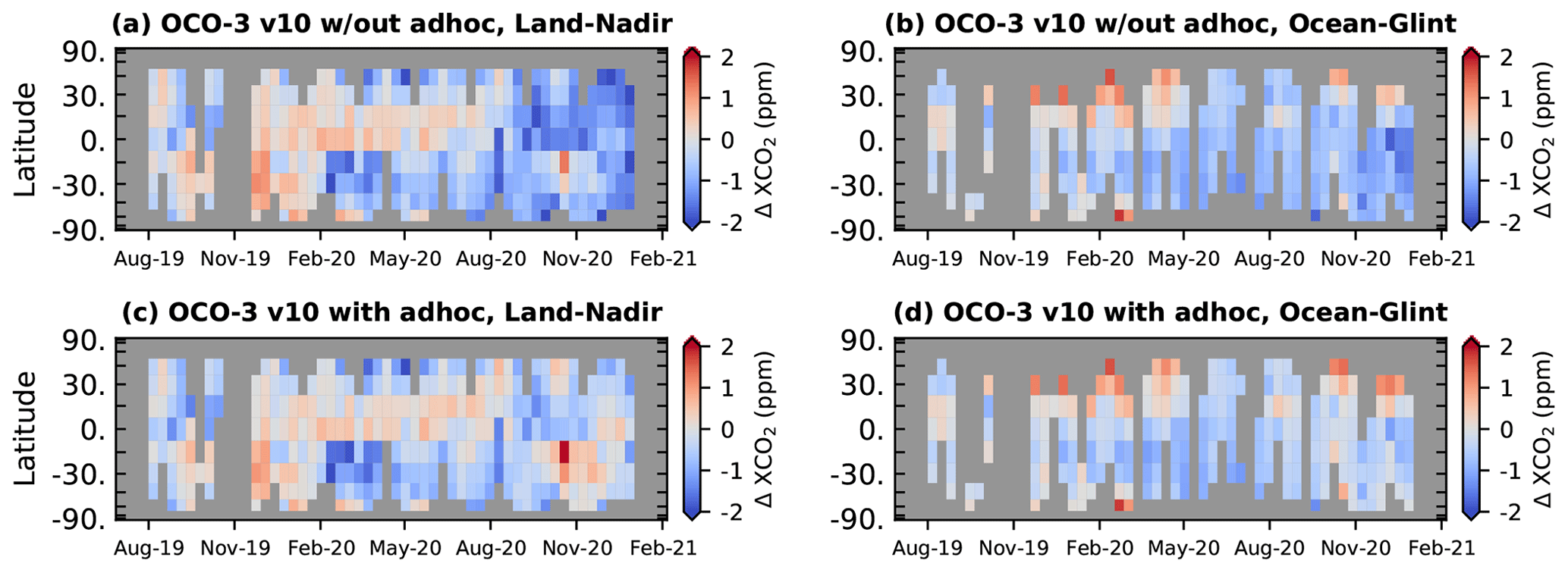
Figure B5The XCO2 signal (OCO-3 − MMM) gridded at 15∘ latitude by 10 d for the time period of August 2019 through December 2020. Panels (a) and (c) show results before and after the ad hoc XCO2 bias correction for land–nadir observations, while panels (b) and (d) are for ocean–glint observations. The ordinate axis is scaled by the cosine of the latitude to elucidate the decreasing fractional surface area of the Earth with increasing latitude. Data cells with fewer than 10 soundings are colored gray.
Figure B5 shows a verification of the OCO-3 XCO2 ad hoc correction compared to the multi-model median (MMM) that was discussed in Sect. 6.2. The top row shows results prior to the ad hoc correction for land–nadir (Fig. B5a) and for ocean–glint (Fig. B5b). Although early in the record the agreement is quite good, a strong, unexpected time divergence is seen in the uncorrected data in the second half of 2020. After application of the ad hoc bias correction, as seen in Fig. B5c for land and Fig. B5d for ocean–glint, the OCO-3 XCO2 is in better agreement with the MMM and is on par with expectations based on previous results from both OCO-2 and GOSAT, e.g., Sect. 6.2 of this work and Sect. 4.4 of Taylor et al. (2022).
B4 OCO-3 v10 XCO2 diurnal signal
The orbit of OCO-3 aboard the ISS precesses in time such that the Equator crossing occurs approximately 20 min earlier each day. This yields observations spanning all daylight hours over the course of a 63 d repeat cycle (Eldering et al., 2019). The semi-diurnal nature of the OCO-3 data has potential to allow for interesting science investigations (e.g., Xiao et al., 2021) that are not possible with data from polar orbiters with a fixed overpass time.
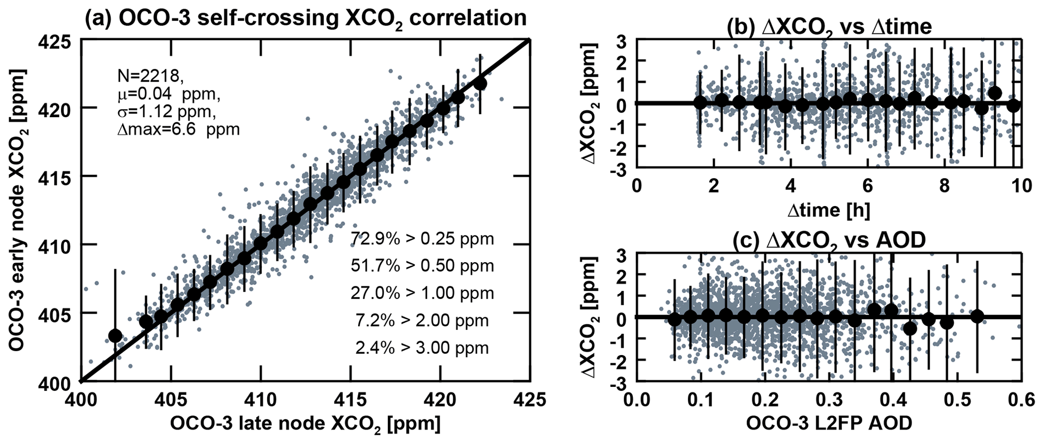
Figure B6Analysis of OCO-3 XCO2 from a set of paired intersecting orbits, i.e., self-crossings, over land. Panel (a) shows the one-to-one correspondence in XCO2 between the early and late orbits. The number of collocations (N), mean (μ), standard deviation (σ), and maximum ΔXCO2 (Δmax) are given in the legend. Also shown in the legend is the percent of the collocations having ΔXCO2 greater than 0.25, 0.5, 1.0, 2.0, and 3.0 ppm. Panel (b) shows the ΔXCO2 versus the time difference between self-crossings. Panel (c) shows the ΔXCO2 versus the L2FP retrieved total aerosol optical depth (combined for the ascending and descending nodes).
Analysis of OCO-3 XCO2 from a set of more than 2000 same-day paired intersecting orbits, i.e., self-crossings, over land is shown in Fig. B6. The time separation between intersecting orbits ranges from 1.5 h up to approximately 10 h, with a spatial coincidence of 25 km radius. The difference in observed XCO2 between overpasses is a combination of random uncertainty driven by instrument calibration and retrieval uncertainties, plus real changes in XCO2. Over a timescale of hours, local variations in XCO2 are due to a combination of (i) synoptic-scale transport, i.e., CO2 weather (Parazoo et al., 2008), (ii) biospheric diurnal effects, i.e., drawdown by the terrestrial biosphere (Keppel-Aleks et al., 2011), and (iii) local point source emissions (e.g., Nassar et al., 2021).
Panel (a) of Fig. B6 shows the one-to-one correspondence in XCO2 between the 2218 pairs of orbits. The mean difference is 0.04 ppm with a 1.1 ppm uncertainty. About one-quarter of the samples have a difference smaller than 0.25 ppm, while one-quarter have a difference larger than 1 ppm, which is near the upper end of expected diurnal changes in the column (Torres et al., 2019). The maximum observed difference is > 6.6 ppm! A test using a tighter spatial collocation of 10 km radius yielded indistinguishable differences, but a reduction in the number of collocations to ≈1850 (results not shown).
Panel (b) of Fig. B6 shows the ΔXCO2 versus the time difference between self-crossings. It might be expected that if the self-crossings were detecting real changes in the column CO2 between overpasses driven by smooth diurnal variations due to biospheric drawdown, then larger ΔXCO2 would be seen at larger Δtime. However, no significant correlation in ΔXCO2 with Δtime is observed. The largest differences in XCO2 are about as likely to occur between two orbits 1.5 h apart as they are to occur between two orbits 8 or 9 h apart.
An effort was made to explore geophysical and retrieval covariates in the observed XCO2 differences. Any significant correlations between ΔXCO2 and L2FP retrieval variables, as is done in the bias correction procedure, could help to understand physical processes, as aerosols are a known source of error in the L2FP (Nelson and O'Dell, 2019; Bell et al., 2023). Figure B6c shows the correlation in ΔXCO2 with the L2FP retrieved total aerosol optical depth (combined for the two overpasses). Although there is a modest increase in spread for higher values of AOD, the median ΔXCO2 values (heavy filled circles with 1σ error bars) show no significant correlation. No other L2FP retrieval variables, e.g., albedos and geometries, were found to correlate with ΔXCO2 (results not shown).
Although additional analysis is warranted, the general conclusion is that the variability in the ΔXCO2 from the self-crossing analysis is dominated by random uncertainties in the measurements and/or the L2FP retrieval. This conclusion is in line with reported XCO2 errors on the order of 0.5 ppm and with the fidelity of the comparisons against truth proxies.
The OCO XCO2 and other retrieval properties are publicly available at the NASA Goddard Earth Science Data and Information Services Center (GES-DISC). The full suite of retrieval products in the standard per-orbit format can be obtained at https://doi.org/10.5067/6SBROTA57TFH (OCO Science Team et al., 2020b) and https://doi.org/10.5067/D9S8ZOCHCADE (OCO Science Team et al., 2021) for OCO-2 and OCO-3, respectively. The Lite files, which include the quality-flagged and bias-corrected estimates of XCO2, can be obtained at https://doi.org/10.5067/E4E140XDMPO2 (OCO Science Team et al., 2020a) and https://doi.org/10.5067/970BCC4DHH24 (OCO Science Team et al., 2022) for OCO-2 and OCO-3, respectively. For OCO-3, researchers are urged to use the v10.4 Lite files and avoid use of the XCO2 values reported in the v10 L2 Standard product, which do not have the ad hoc bias correction applied.
The TCCON data for individual stations are referenced in Table 3 and are available on the CaltechDATA site (https://data.caltech.edu/, last access: 21 June 2023). CarbonTracker CT-NRT.v2019-2 and CT-NRT.v2021-3 results are provided by NOAA ESRL, Boulder, Colorado, USA, from the website at https://carbontracker.noaa.gov (last access: 21 June 2023). The Jena-CarboScope model data are available at http://www.bgc-jena.mpg.de/CarboScope (last access: 21 June 2023). The Copernicus Atmosphere Monitoring Service (CAMS) CAMS-INV model data were obtained from https://ads.atmosphere.copernicus.eu/cdsapp#!/dataset/cams-global-greenhouse-gas-inversion?tab=overview (last access: 21 June 2023), while the CAMS-REAN data were obtained from https://ads.atmosphere.copernicus.eu/cdsapp#!/dataset/cams-global-ghg-reanalysis-egg4?tab=overview (last access: 21 June 2023). The UoL model data are available at https://www.geos.ed.ac.uk/~lfeng/ (last access: 21 June 2023). The GEOS data used in this study were provided by the Global Modeling and Assimilation Office (GMAO) at NASA Goddard Space Flight Center.
TET conceptualized the study, performed the data analysis, generated the graphics, and wrote the paper. CWO'D helped conceptualize the study, led the ACOS L2FP retrieval algorithm development, performed the quality filtering and bias correction, helped with data analysis, and edited an early draft of the paper. CB, LC, DF, VH, RL, YM, GRK, RR, and SY performed instrument calibration required for accurate retrievals of XCO2. JZ performed the geolocation of the soundings. BD and FO developed and provided the spectroscopic lookup tables that are crucial for accurate retrievals of XCO2. BF, MK, LK, TK, AL, JL, LM, GM, AM, RRN, GO, PS, GS, and POW all contributed in various ways to OCO operations, the v10 ACOS L2FP algorithm testing and development, and the v10 quality filtering and bias correction procedure. AlC, CC, LD, and CT performed the data testing and maintained the operational pipeline required to produce the XCO2 products. DB provided the 10 s average XCO2 files used in the evaluation against models and provided valuable insight into the OCO v10 XCO2 products during and after development. FC, LF, PIP, and BW provided model data used in the quality filtering, bias correction, and evaluation of the v10 XCO2. VHP and AbC are the current project scientists for OCO-2 and OCO-3, respectively, while MG and AE were the former project scientists for OCO-2 and OCO-3, respectively. JL is the current OCO-2/3 science team lead, while DC was the former OCO-2/3 science team lead. DC also edited a mature version of the paper. All coauthors reviewed and provided comments on the draft paper prior to submission.
At least one of the (co-)authors is a member of the editorial board of Atmospheric Measurement Techniques. The peer-review process was guided by an independent editor, and the authors also have no other competing interests to declare.
Publisher's note: Copernicus Publications remains neutral with regard to jurisdictional claims in published maps and institutional affiliations.
A portion of this research was carried out at the Jet Propulsion Laboratory, California Institute of Technology, under contract with the National Aeronautics and Space Administration (80NM0018D0004). Government sponsorship is acknowledged. The CSU/CIRA contribution to this work was supported by JPL subcontracts 1439002 (OCO-2) and 1557985 (OCO-3). Aronne Merrelli's contributions to this work were supported by JPL subcontract 1577173. Paul I. Palmer and Liang Feng acknowledge support from the UK National Centre for Earth Observation funded by the National Environment Research Council (NE/R016518/1). We gratefully acknowledge the use of TCCON data in this work. We thank the two anonymous reviewers for their time to provide very useful comments on the paper. We also thank the journal editor, Joanna Joiner, for her willingness to oversee the review process.
This research has been supported by the National Aeronautics and Space Administration (grant no. 80NM0018D0004), JPL (subcontracts 1439002 (OCO-2), 1557985 (OCO-3), and 1577173), and the UK National Centre for Earth Observation funded by the National Environment Research Council (grant no. NE/R016518/1).
This paper was edited by Joanna Joiner and reviewed by two anonymous referees.
Agustí-Panareda, A., Massart, S., Chevallier, F., Boussetta, S., Balsamo, G., Beljaars, A., Ciais, P., Deutscher, N. M., Engelen, R., Jones, L., Kivi, R., Paris, J.-D., Peuch, V.-H., Sherlock, V., Vermeulen, A. T., Wennberg, P. O., and Wunch, D.: Forecasting global atmospheric CO2, Atmos. Chem. Phys., 14, 11959–11983, https://doi.org/10.5194/acp-14-11959-2014, 2014. a
Archer, D., Eby, M., Brovkin, V., Ridgwell, A., Cao, L., Mikolajewicz, U., Caldeira, K., Matsumoto, K., Munhoven, G., Montenegro, A., and Tokos, K.: Atmospheric Lifetime of Fossil Fuel Carbon Dioxide, Annu. Rev. Earth Pl. Sc., 37, 117–134, https://doi.org/10.1146/annurev.earth.031208.100206, 2009. a
Baker, D. F., Bell, E., Davis, K. J., Campbell, J. F., Lin, B., and Dobler, J.: A new exponentially decaying error correlation model for assimilating OCO-2 column-average CO2 data using a length scale computed from airborne lidar measurements, Geosci. Model Dev., 15, 649–668, https://doi.org/10.5194/gmd-15-649-2022, 2022. a, b
Basu, S., Guerlet, S., Butz, A., Houweling, S., Hasekamp, O., Aben, I., Krummel, P., Steele, P., Langenfelds, R., Torn, M., Biraud, S., Stephens, B., Andrews, A., and Worthy, D.: Global CO2 fluxes estimated from GOSAT retrievals of total column CO2, Atmos. Chem. Phys., 13, 8695–8717, https://doi.org/10.5194/acp-13-8695-2013, 2013. a
Bell, E., O'Dell, C. W., Davis, K. J., Campbell, J., Browell, E., Scott Denning, A., Dobler, J., Erxleben, W., Fan, T.-F., Kooi, S., Lin, B., Pal, S., and Weir, B.: Evaluation of OCO-2 XCO2 variability at local and synoptic scales using lidar and in situ observations from the ACT-America campaigns, J. Geophys. Res.-Atmos., 125, e2019JD031400, https://doi.org/10.1029/2019JD031400, 2020. a, b
Bell, E., O'Dell, C. W., Taylor, T. E., Merrelli, A., Nelson, R. R., Kiel, M., Eldering, A., Rosenberg, R., and Fisher, B.: Exploring bias in the OCO-3 snapshot area mapping mode via geometry, surface, and aerosol effects, Atmos. Meas. Tech., 16, 109–133, https://doi.org/10.5194/amt-16-109-2023, 2023. a, b
Blumenstock, T., Hase, F., Schneider, M., Garcia, O. E., and Sepulveda, E.: TCCON data from Izana (ES), Release GGG2014R1, TCCON data archive, CaltechDATA [data set], https://doi.org/10.14291/TCCON.GGG2014.IZANA01.R1, 2017. a
Bruegge, C. J., Crisp, D., Helmlinger, M. C., Kataoka, F., Kuze, A., Lee, R. A., McDuffie, J. L., Rosenberg, R. A., Schwandner, F. M., Shiomi, K., and Yu, S.: Vicarious Calibration of Orbiting Carbon Observatory-2, IEEE T. Geosci. Remote, 57, 5135–5145, https://doi.org/10.1109/TGRS.2019.2897068, 2019. a
Buchwitz, M., Reuter, M., Schneising, O., Hewson, W., Detmers, R., Boesch, H., Hasekamp, O., Aben, I., Bovensmann, H., Burrows, J., Butz, A., Chevallier, F., Dils, B., Frankenberg, C., Heymann, J., Lichtenberg, G., De Mazière, M., Notholt, J., Parker, R., Warneke, T., Zehner, C., Griffith, D., Deutscher, N., Kuze, A., Suto, H., and Wunch, D.: Global satellite observations of column-averaged carbon dioxide and methane: The GHG-CCI XCO2 and XCH4 CRDP3 data set, Remote Sensing of Environment, 203, 276–295, https://doi.org/10.1016/j.rse.2016.12.027, 2017. a
Buchwitz, M., Reuter, M., Schneising, O., Noël, S., Gier, B., Bovensmann, H., Burrows, J. P., Boesch, H., Anand, J., Parker, R. J., Somkuti, P., Detmers, R. G., Hasekamp, O. P., Aben, I., Butz, A., Kuze, A., Suto, H., Yoshida, Y., Crisp, D., and O'Dell, C.: Computation and analysis of atmospheric carbon dioxide annual mean growth rates from satellite observations during 2003–2016, Atmos. Chem. Phys., 18, 17355–17370, https://doi.org/10.5194/acp-18-17355-2018, 2018. a, b
Byrne, B., Liu, J., Lee, M., Yin, Y., Bowman, K. W., Miyazaki, K., Norton, A. J., Joiner, J., Pollard, D. F., Griffith, D. W. T., Velazco, V. A., Deutscher, N. M., Jones, N. B., and Paton-Walsh, C.: The Carbon Cycle of Southeast Australia During 2019–2020: Drought, Fires, and Subsequent Recovery, AGU Advances, 2, e2021AV000469, https://doi.org/10.1029/2021AV000469, 2021. a, b
Byrne, B., Liu, J., Yi, Y., Chatterjee, A., Basu, S., Cheng, R., Doughty, R., Chevallier, F., Bowman, K. W., Parazoo, N. C., Crisp, D., Li, X., Xiao, J., Sitch, S., Guenet, B., Deng, F., Johnson, M. S., Philip, S., McGuire, P. C., and Miller, C. E.: Multi-year observations reveal a larger than expected autumn respiration signal across northeast Eurasia, Biogeosciences, 19, 4779–4799, https://doi.org/10.5194/bg-19-4779-2022, 2022. a, b
Byrne, B., Baker, D. F., Basu, S., Bertolacci, M., Bowman, K. W., Carroll, D., Chatterjee, A., Chevallier, F., Ciais, P., Cressie, N., Crisp, D., Crowell, S., Deng, F., Deng, Z., Deutscher, N. M., Dubey, M. K., Feng, S., García, O. E., Griffith, D. W. T., Herkommer, B., Hu, L., Jacobson, A. R., Janardanan, R., Jeong, S., Johnson, M. S., Jones, D. B. A., Kivi, R., Liu, J., Liu, Z., Maksyutov, S., Miller, J. B., Miller, S. M., Morino, I., Notholt, J., Oda, T., O'Dell, C. W., Oh, Y.-S., Ohyama, H., Patra, P. K., Peiro, H., Petri, C., Philip, S., Pollard, D. F., Poulter, B., Remaud, M., Schuh, A., Sha, M. K., Shiomi, K., Strong, K., Sweeney, C., Té, Y., Tian, H., Velazco, V. A., Vrekoussis, M., Warneke, T., Worden, J. R., Wunch, D., Yao, Y., Yun, J., Zammit-Mangion, A., and Zeng, N.: National CO2 budgets (2015–2020) inferred from atmospheric CO2 observations in support of the global stocktake, Earth Syst. Sci. Data, 15, 963–1004, https://doi.org/10.5194/essd-15-963-2023, 2023. a, b, c, d
Chahine, M., Chen, L., Dimotakis, P., Jiang, X., Li, Q., Olsen, E., Pagano, T., Randerson, J., and Yung, Y.: Satellite remote sensing of mid-tropospheric CO2, Geophys. Res. Lett., 35, L17807, https://doi.org/10.1029/2008GL035022, 2008. a
Chatterjee, A., Gierach, M. M., Sutton, A. J., Feely, R. A., Crisp, D., Eldering, A., Gunson, M. R., O'Dell, C. W., Stephens, B. B., and Schimel, D. S.: Influence of El Niño on atmospheric CO2 over the tropical Pacific Ocean: Findings from NASA's OCO-2 mission, Science, 358, eaam5776, https://doi.org/10.1126/science.aam5776, 2017. a
Chatterjee, A., Payne, V., Eldering, A., Rosenberg, R., Kiel, M., Fisher, B., Nelson, R., Dang, L., Rodrigues, G. K., O'Dell, C., Taylor, T., and Osterman, G.: Orbiting Carbon Observatory-2 & 3 Data Quality Statement, v10, v10r, v10.4, Tech. rep., Jet Propulsion Laboratory, https://docserver.gesdisc.eosdis.nasa.gov/public/project/OCO/OCO3_L2_DQ_Statement_v10_v104.pdf (last access: 15 June 2023), 2022. a, b, c, d
Chevallier, F.: Validation report for the CO2 fluxes estimated by atmospheric inversion, v18r2, version 1.0, Copernicus Atmosphere Monitoring Service, https://atmosphere.copernicus.eu/sites/default/files/2019-08/CAMS73_2018SC1_D73.1.4.1-2018-v1_201907_v1.pdf (last access: 15 June 2023), 2021. a
Chevallier, F., Engelen, R. J., and Peylin, P.: The contribution of AIRS data to the estimation of CO2 sources and sinks, Geophys. Res. Lett., 32, L23801, https://doi.org/10.1029/2005GL024229, 2005. a
Chevallier, F., Bréon, F.-M., and Rayner, P. J.: Contribution of the Orbiting Carbon Observatory to the estimation of CO2 sources and sinks: Theoretical study in a variational data assimilation framework, J. Geophys. Res.-Atmos., 112, D09307, https://doi.org/10.1029/2006JD007375, 2007. a
Chevallier, F., Ciais, P., Conway, T. J., Aalto, T., Anderson, B. E., Bousquet, P., Brunke, E. G., Ciattaglia, L., Esaki, Y., Fröhlich, M., Gomez, A., Gomez-Pelaez, A. J., Haszpra, L., Krummel, P. B., Langenfelds, R. L., Leuenberger, M., Machida, T., Maignan, F., Matsueda, H., Morguí, J. A., Mukai, H., Nakazawa, T., Peylin, P., Ramonet, M., Rivier, L., Sawa, Y., Schmidt, M., Steele, L. P., Vay, S. A., Vermeulen, A. T., Wofsy, S., and Worthy, D.: CO2 surface fluxes at grid point scale estimated from a global 21 year reanalysis of atmospheric measurements, J. Geophys. Res.-Atmos., 115, D21307, https://doi.org/10.1029/2010JD013887, 2010. a
Chevallier, F., Palmer, P. I., Feng, L., Boesch, H., O'Dell, C. W., and Bousquet, P.: Toward robust and consistent regional CO2 flux estimates from in situ and spaceborne measurements of atmospheric CO2, Geophys. Res. Lett., 41, 1065–1070, https://doi.org/10.1002/2013GL058772, 2014. a
Chevallier, F., Broquet, G., Zheng, B., Ciais, P., and Eldering, A.: Large CO2 Emitters as Seen From Satellite: Comparison to a Gridded Global Emission Inventory, Geophys. Res. Lett., 49, e2021GL097540, https://doi.org/10.1029/2021GL097540, 2022. a, b
Ciais, P., Dolman, A. J., Bombelli, A., Duren, R., Peregon, A., Rayner, P. J., Miller, C., Gobron, N., Kinderman, G., Marland, G., Gruber, N., Chevallier, F., Andres, R. J., Balsamo, G., Bopp, L., Bréon, F.-M., Broquet, G., Dargaville, R., Battin, T. J., Borges, A., Bovensmann, H., Buchwitz, M., Butler, J., Canadell, J. G., Cook, R. B., DeFries, R., Engelen, R., Gurney, K. R., Heinze, C., Heimann, M., Held, A., Henry, M., Law, B., Luyssaert, S., Miller, J., Moriyama, T., Moulin, C., Myneni, R. B., Nussli, C., Obersteiner, M., Ojima, D., Pan, Y., Paris, J.-D., Piao, S. L., Poulter, B., Plummer, S., Quegan, S., Raymond, P., Reichstein, M., Rivier, L., Sabine, C., Schimel, D., Tarasova, O., Valentini, R., Wang, R., van der Werf, G., Wickland, D., Williams, M., and Zehner, C.: Current systematic carbon-cycle observations and the need for implementing a policy-relevant carbon observing system, Biogeosciences, 11, 3547–3602, https://doi.org/10.5194/bg-11-3547-2014, 2014. a
Coddington, O. M., Richard, E. C., Harber, D., Pilewskie, P., Woods, T. N., Chance, K., Liu, X., and Sun, K.: The TSIS-1 Hybrid Solar Reference Spectrum, Geophys. Res. Lett., 48, e2020GL091709, https://doi.org/10.1029/2020GL091709, 2021. a
Connor, B., Bösch, H., McDuffie, J., Taylor, T., Fu, D., Frankenberg, C., O'Dell, C., Payne, V. H., Gunson, M., Pollock, R., Hobbs, J., Oyafuso, F., and Jiang, Y.: Quantification of uncertainties in OCO-2 measurements of XCO2: simulations and linear error analysis, Atmos. Meas. Tech., 9, 5227–5238, https://doi.org/10.5194/amt-9-5227-2016, 2016. a
Connor, B. J., Boesch, H., Toon, G., Sen, B., Miller, C., and Crisp, D.: Orbiting Carbon Observatory: Inverse method and prospective error analysis, J. Geophys. Res.-Atmos., 113, D05305, https://doi.org/10.1029/2006JD008336, 2008. a, b
Conway, T. J., Tans, P. P., Waterman, L. S., Thoning, K. W., Kitzis, D. R., Masarie, K. A., and Zhang, N.: Evidence for interannual variability of the carbon cycle from the National Oceanic and Atmospheric Administration/Climate Monitoring and Diagnostics Laboratory Global Air Sampling Network, J. Geophys. Res.-Atmos., 99, 22831–22855, https://doi.org/10.1029/94JD01951, 1994. a
Crisp, D., Pollock, H. R., Rosenberg, R., Chapsky, L., Lee, R. A. M., Oyafuso, F. A., Frankenberg, C., O'Dell, C. W., Bruegge, C. J., Doran, G. B., Eldering, A., Fisher, B. M., Fu, D., Gunson, M. R., Mandrake, L., Osterman, G. B., Schwandner, F. M., Sun, K., Taylor, T. E., Wennberg, P. O., and Wunch, D.: The on-orbit performance of the Orbiting Carbon Observatory-2 (OCO-2) instrument and its radiometrically calibrated products, Atmos. Meas. Tech., 10, 59–81, https://doi.org/10.5194/amt-10-59-2017, 2017. a, b, c, d, e
Crisp, D., Meijer, Y., Munro, R., Bowman, K., and Chatterjee, A.: A constellation architecture for monitoring carbon dioxide and methane from space, Tech. rep., Committee on Earth Observation Satellites, https://ceos.org/document_management/Virtual_Constellations/ACC/Documents/CEOS_AC-VC_GHG_White_Paper_Publication_Draft2_20181111.pdf (last access: 15 June 2023), 2018. a
Crisp, D., O'Dell, C., Eldering, A., Fisher, B., Oyafuso, F., Payne, V., Drouin, B., Toon, G., Laughner, J., Somkuti, P., McGarragh, G., Merrelli, A., Nelson, R., Gunson, M., Frankenberg, C., Osterman, G., Boesch, H., Brown, L., Castano, R., Christi, M., Connor, B., McDuffie, J., Miller, C., Natraj, V., O'Brien, D., Polonsky, I., Smyth, M., Thompson, D., and Granat, R.: Orbiting Carbon Observatory-2 & 3 Level 2 Full Physics Retrieval Algorithm Theoretical Basis, v10, Tech. rep., Jet Propulsion Laboratory, https://docserver.gesdisc.eosdis.nasa.gov/public/project/OCO/OCO_L2_ATBD.pdf (last access: 15 June 2023), 2020. a, b, c
Crisp, D., Rosenberg, R., Chapsky, L., Rodrigues, G. R. K., Lee, R., Merrelli, A., Osterman, G., Oyafuso, F., Pollock, R., Spiers, G., Yu, S., Zong, J., and Eldering, A.: Orbiting Carbon Observatory-2 & 3 Level 1B Algorithm Theoretical Basis, v10, Tech. rep., Jet Propulsion Laboratory, https://docserver.gesdisc.eosdis.nasa.gov/public/project/OCO/OCO_L1B_ATBD.pdf (last access: 15 June 2023), 2021. a, b
Crisp, D., Dolman, H., Tanhua, T., McKinley, G. A., Hauck, J., Bastos, A., Sitch, S., Eggleston, S., and Aich, V.: How Well Do We Understand the Land-Ocean-Atmosphere Carbon Cycle?, Rev. Geophys., 60, e2021RG000736, https://doi.org/10.1029/2021RG000736, 2022. a
Crowell, S., Baker, D., Schuh, A., Basu, S., Jacobson, A. R., Chevallier, F., Liu, J., Deng, F., Feng, L., McKain, K., Chatterjee, A., Miller, J. B., Stephens, B. B., Eldering, A., Crisp, D., Schimel, D., Nassar, R., O'Dell, C. W., Oda, T., Sweeney, C., Palmer, P. I., and Jones, D. B. A.: The 2015–2016 carbon cycle as seen from OCO-2 and the global in situ network, Atmos. Chem. Phys., 19, 9797–9831, https://doi.org/10.5194/acp-19-9797-2019, 2019. a, b
De Mazière, M., Sha, M. K., Desmet, F., Hermans, C., Scolas, F., Kumps, N., Metzger, J.-M., Duflot, V., and Cammas, J.-P.: TCCON data from Réunion Island (RE), Release GGG2014.R1, TCCON data archive, CaltechDATA [data set], https://doi.org/10.14291/TCCON.GGG2014.REUNION01.R1, 2017. a
Deutscher, N. M., Notholt, J., Messerschmidt, J., Weinzierl, C., Warneke, T., Petri, C., and Grupe, P.: TCCON data from Bialystok (PL), Release GGG2014.R2, TCCON data archive, CaltechDATA [data set], https://doi.org/10.14291/TCCON.GGG2014.BIALYSTOK01.R2, 2017. a
Dlugokencky, E. and Tans, P.: Trends in atmospheric carbon dioxide, NOAA/GML, https://gml.noaa.gov/ccgg/trends/ (last access: 15 June 2023), 2022. a
Doughty, R., Kurosu, T. P., Parazoo, N., Köhler, P., Wang, Y., Sun, Y., and Frankenberg, C.: Global GOSAT, OCO-2, and OCO-3 solar-induced chlorophyll fluorescence datasets, Earth Syst. Sci. Data, 14, 1513–1529, https://doi.org/10.5194/essd-14-1513-2022, 2022. a, b
Drouin, B. J., Benner, D. C., Brown, L. R., Cich, M. J., Crawford, T. J., Devi, V. M., Guillaume, A., Hodges, J. T., Mlawer, E. J., Robichaud, D. J., Oyafuso, F., Payne, V. H., Sung, K., Wishnow, E. H., and Yu, S.: Multispectrum analysis of the oxygen A-band, J. Quant. Spectrosc. Ra., 186, 118–138, https://doi.org/10.1016/j.jqsrt.2016.03.037, 2017. a, b
Eldering, A., O'Dell, C. W., Wennberg, P. O., Crisp, D., Gunson, M. R., Viatte, C., Avis, C., Braverman, A., Castano, R., Chang, A., Chapsky, L., Cheng, C., Connor, B., Dang, L., Doran, G., Fisher, B., Frankenberg, C., Fu, D., Granat, R., Hobbs, J., Lee, R. A. M., Mandrake, L., McDuffie, J., Miller, C. E., Myers, V., Natraj, V., O'Brien, D., Osterman, G. B., Oyafuso, F., Payne, V. H., Pollock, H. R., Polonsky, I., Roehl, C. M., Rosenberg, R., Schwandner, F., Smyth, M., Tang, V., Taylor, T. E., To, C., Wunch, D., and Yoshimizu, J.: The Orbiting Carbon Observatory-2: first 18 months of science data products, Atmos. Meas. Tech., 10, 549–563, https://doi.org/10.5194/amt-10-549-2017, 2017. a
Eldering, A., Taylor, T. E., O'Dell, C. W., and Pavlick, R.: The OCO-3 mission: measurement objectives and expected performance based on 1 year of simulated data, Atmos. Meas. Tech., 12, 2341–2370, https://doi.org/10.5194/amt-12-2341-2019, 2019. a, b
Feist, D. G., Arnold, S. G., John, N., and Geibel, M. C.: TCCON data from Ascension Island (SH), Release GGG2014.R0, TCCON data archive, CaltechDATA [data set], https://doi.org/10.14291/TCCON.GGG2014.ASCENSION01.R0/1149285, 2017. a
Feng, L., Palmer, P. I., Bösch, H., and Dance, S.: Estimating surface CO2 fluxes from space-borne CO2 dry air mole fraction observations using an ensemble Kalman Filter, Atmos. Chem. Phys., 9, 2619–2633, https://doi.org/10.5194/acp-9-2619-2009, 2009. a
Feng, L., Palmer, P. I., Parker, R. J., Deutscher, N. M., Feist, D. G., Kivi, R., Morino, I., and Sussmann, R.: Estimates of European uptake of CO2 inferred from GOSAT X retrievals: sensitivity to measurement bias inside and outside Europe, Atmos. Chem. Phys., 16, 1289–1302, https://doi.org/10.5194/acp-16-1289-2016, 2016. a
Frankenberg, C., Platt, U., and Wagner, T.: Iterative maximum a posteriori (IMAP)-DOAS for retrieval of strongly absorbing trace gases: Model studies for CH4 and CO2 retrieval from near infrared spectra of SCIAMACHY onboard ENVISAT, Atmos. Chem. Phys., 5, 9–22, https://doi.org/10.5194/acp-5-9-2005, 2005. a
Frankenberg, C., O'Dell, C., Guanter, L., and McDuffie, J.: Remote sensing of near-infrared chlorophyll fluorescence from space in scattering atmospheres: implications for its retrieval and interferences with atmospheric CO2 retrievals, Atmos. Meas. Tech., 5, 2081–2094, https://doi.org/10.5194/amt-5-2081-2012, 2012. a
Friedlingstein, P., O'Sullivan, M., Jones, M. W., Andrew, R. M., Gregor, L., Hauck, J., Le Quéré, C., Luijkx, I. T., Olsen, A., Peters, G. P., Peters, W., Pongratz, J., Schwingshackl, C., Sitch, S., Canadell, J. G., Ciais, P., Jackson, R. B., Alin, S. R., Alkama, R., Arneth, A., Arora, V. K., Bates, N. R., Becker, M., Bellouin, N., Bittig, H. C., Bopp, L., Chevallier, F., Chini, L. P., Cronin, M., Evans, W., Falk, S., Feely, R. A., Gasser, T., Gehlen, M., Gkritzalis, T., Gloege, L., Grassi, G., Gruber, N., Gürses, Ö., Harris, I., Hefner, M., Houghton, R. A., Hurtt, G. C., Iida, Y., Ilyina, T., Jain, A. K., Jersild, A., Kadono, K., Kato, E., Kennedy, D., Klein Goldewijk, K., Knauer, J., Korsbakken, J. I., Landschützer, P., Lefèvre, N., Lindsay, K., Liu, J., Liu, Z., Marland, G., Mayot, N., McGrath, M. J., Metzl, N., Monacci, N. M., Munro, D. R., Nakaoka, S.-I., Niwa, Y., O'Brien, K., Ono, T., Palmer, P. I., Pan, N., Pierrot, D., Pocock, K., Poulter, B., Resplandy, L., Robertson, E., Rödenbeck, C., Rodriguez, C., Rosan, T. M., Schwinger, J., Séférian, R., Shutler, J. D., Skjelvan, I., Steinhoff, T., Sun, Q., Sutton, A. J., Sweeney, C., Takao, S., Tanhua, T., Tans, P. P., Tian, X., Tian, H., Tilbrook, B., Tsujino, H., Tubiello, F., van der Werf, G. R., Walker, A. P., Wanninkhof, R., Whitehead, C., Willstrand Wranne, A., Wright, R., Yuan, W., Yue, C., Yue, X., Zaehle, S., Zeng, J., and Zheng, B.: Global Carbon Budget 2022, Earth Syst. Sci. Data, 14, 4811–4900, https://doi.org/10.5194/essd-14-4811-2022, 2022. a
Gelaro, R., McCarty, W., Suárez, M. J., Todling, R., Molod, A., Takacs, L., Randles, C. A., Darmenov, A., Bosilovich, M. G., Reichle, R., Wargan, K., Coy, L., Cullather, R., Draper, C., Akella, S., Buchard, V., Conaty, A., da Silva, A. M., Gu, W., Kim, G.-K., Koster, R., Lucchesi, R., Merkova, D., Nielsen, J. E., Partyka, G., Pawson, S., Putman, W., Rienecker, M., Schubert, S. D., Sienkiewicz, M., and Zhao, B.: The Modern-Era Retrospective Analysis for Research and Applications, Version 2 (MERRA-2), J. Climate, 30, 5419–5454, https://doi.org/10.1175/JCLI-D-16-0758.1, 2017. a
Goo, T.-Y., Oh, Y.-S., and Velazco, V. A.: TCCON data from Anmeyondo (KR), Release GGG2014.R0, TCCON data archive, CaltechDATA [data set], https://doi.org/10.14291/TCCON.GGG2014.ANMEYONDO01.R0/1149284, 2017. a
Griffith, D. W., Deutscher, N. M., Velazco, V. A., Wennberg, P. O., Yavin, Y., Aleks, G. K., Washenfelder, R. A., Toon, G. C., Blavier, J.-F., Murphy, C., Jones, N., Kettlewell, G., Connor, B. J., Macatangay, R., Roehl, C., Ryczek, M., Glowacki, J., Culgan, T., and Bryant, G.: TCCON data from Darwin (AU), Release GGG2014R0, TCCON data archive, CaltechDATA [data set], https://doi.org/10.14291/tccon.ggg2014.darwin01.R0/1149290, 2014a. a
Griffith, D. W., Velazco, V. A., Deutscher, N. M., Murphy, C., Jones, N., Wilson, S., Macatangay, R., Kettlewell, G., Buchholz, R. R., and Riggenbach, M.: TCCON data from Wollongong (AU), Release GGG2014R0, TCCON data archive, CaltechDATA [data set], https://doi.org/10.14291/tccon.ggg2014.wollongong01.R0/1149291, 2014b. a
Gurney, K. R., Law, R. M., Denning, S., Rayner, P. J., Baker, D., Bousquet, P., Bruhwiler, L., Chen, Y.-H., Ciais, P., Fan, S., Fung, I. Y., Gloor, M., Heimann, M., Higuchi, K., John, J., Maki, T., Maksyutov, S., Masarie, K., Peylin, P., Prather, M., Pak, B. C., Randerson, J., Sarmiento, J., Taguchi, S., Takahashi, T., and Yuen, C.-W.: Towards robust regional estimates of CO2 sources and sinks using atmospheric transport models, Nature, 415, 626–630, https://doi.org/10.1038/415626a, 2002. a
Hase, F., Blumenstock, T., Dohe, S., Gross, J., and Kiel, M.: TCCON data from Karlsruhe (DE), Release GGG2014R1, TCCON data archive, CaltechDATA [data set], https://doi.org/10.14291/tccon.ggg2014.karlsruhe01.R1/1182416, 2015. a
Hobbs, J., Braverman, A., Cressie, N., Granat, R., and Gunson, M.: Simulation-Based Uncertainty Quantification for Estimating Atmospheric CO2 from Satellite Data, SIAM/ASA Journal on Uncertainty Quantification, 5, 956–985, https://doi.org/10.1137/16M1060765, 2017. a
Iraci, L. T., Podolske, J., Hillyard, P. W., Roehl, C., Wennberg, P. O., Blavier, J.-F., Allen, N., Wunch, D., Osterman, G. B., and Albertson, R.: TCCON data from Edwards (US), Release GGG2014R1, TCCON data archive, CaltechDATA [data set], https://doi.org/10.14291/tccon.ggg2014.edwards01.R1/1255068, 2016. a
Jacobs, N., Simpson, W. R., Wunch, D., O'Dell, C. W., Osterman, G. B., Hase, F., Blumenstock, T., Tu, Q., Frey, M., Dubey, M. K., Parker, H. A., Kivi, R., and Heikkinen, P.: Quality controls, bias, and seasonality of CO2 columns in the boreal forest with Orbiting Carbon Observatory-2, Total Carbon Column Observing Network, and EM27/SUN measurements, Atmos. Meas. Tech., 13, 5033–5063, https://doi.org/10.5194/amt-13-5033-2020, 2020. a
Jacobson, A. R., Schuldt, K. N., Miller, J. B., Tans, P., Andrews, A., Mund, J., Aalto, T., Abshire, J. B., Aikin, K., Aoki, S., Apadula, F., Baier, B., Bakwin, P., Bartyzel, J., Bentz, G., Bergamaschi, P., Beyersdorf, A., Biermann, T., Biraud, S. C., Bowling, D., Brailsford, G., Van Den Bulk, P., Chen, G., Chen, H., Chmura, L., Clark, S., Coletta, J. D., Colomb, A., Commane, R., Conil, S., Cox, A., Cristofanelli, P., Cuevas, E., Curcoll, R., Daube, B., Davis, K., Delmotte, M., DiGangi, J. P., Van Dinther, D., Dlugokencky, E., Elkins, J. W., Emmenegger, L., Fischer, M. L., Forster, G., Frumau, A., Galkowski, M., Gatti, L. V., Gheusi, F., Gloor, E., Gomez-Trueba, V., Goto, D., Griffis, T., Hammer, S., Hanson, C., Haszpra, L., Hatakka, J., Heliasz, M., Hensen, A., Hermanssen, O., Hintsa, E., Holst, J., Jaffe, D., Joubert, W., Karion, A., Kawa, S. R., Kazan, V., Keeling, R., Keronen, P., Kolari, P., Kominkova, K., Kort, E., Krummel, P., Kubistin, D., Labuschagne, C., Langenfelds, R., Laurent, O., Laurila, T., Lauvaux, T., Law, B., Lee, J., Lehner, I., Leuenberger, M., Levin, I., Levula, J., Lin, J., Lindauer, M., Loh, Z., Lopez, M., Machida, T., Mammarella, I., Manca, G., Manning, A., Manning, A., Marek, M. V., Martin, M. Y., Matsueda, H., De Maziäre, M., McKain, K., Meijer, H., Meinhardt, F., Merchant, L., Mihalopoulos, N., Miles, N., Miller, C. E., Mitchell, L., Malder, M., Montzka, S., Moore, F., Morgan, E., Morgui, J.-A., Morimoto, S., Maeller-Williams, J., Munger, B., Myhre, C. L., Necki, J., Newman, S., Nichol, S., Niwa, Y., O'Doherty, S., Paplawsky, B., Peischl, J., Peltola, O., Piacentino, S., Pichon, J. M., Piper, S., Plass-Duelmer, C., Plass-Duelmer, C., Ramonet, M., Ramos, R., Reyes-Sanchez, E., Richardson, S., Riris, H., Rivas, P. P., Ryerson, T., Saito, K., Sargent, M., Di Sarra, A. G., Sawa, Y., Say, D., Scheeren, B., Schmidt, M., Schumacher, M., Sha, M. K., Shepson, P., Shook, M., Sloop, C. D., Smith, P., Steinbacher, M., Stephens, B., Sweeney, C., Thoning, K., Torn, M., Tarseth, K., Trisolino, P., Turnbull, J., Vermeulen, A., Viner, B., Vitkova, G., Walker, S., De Wekker, S., Wofsy, S., Worthy, D., Young, D., and Zimnoch, M.: CarbonTracker Near-Real Time, NOAA Earth System Research Laboratory, Global Monitoring Division, CT-NRT.v2021-3, https://doi.org/10.25925/ED7S-M661, 2021. a
Janssens-Maenhout, G., Pinty, B., Dowell, M., Zunker, H., Andersson, E., Balsamo, G., Bézy, J.-L., Brunhes, T., Bösch, H., Bojkov, B., Brunner, D., Buchwitz, M., Crisp, D., Ciais, P., Counet, P., Dee, D., van der Gon, H. D., Dolman, H., Drinkwater, M. R., Dubovik, O., Engelen, R., Fehr, T., Fernandez, V., Heimann, M., Holmlund, K., Houweling, S., Husband, R., Juvyns, O., Kentarchos, A., Landgraf, J., Lang, R., Löscher, A., Marshall, J., Meijer, Y., Nakajima, M., Palmer, P. I., Peylin, P., Rayner, P., Scholze, M., Sierk, B., Tamminen, J., and Veefkind, P.: Toward an operational anthropogenic CO2 emissions monitoring and verification support capacity, B. Am. Meteorol. Soc., 101, E1439–E1451, https://doi.org/10.1175/BAMS-D-19-0017.1, 2020. a
Jiang, F., Ju, W., He, W., Wu, M., Wang, H., Wang, J., Jia, M., Feng, S., Zhang, L., and Chen, J. M.: A 10-year global monthly averaged terrestrial net ecosystem exchange dataset inferred from the ACOS GOSAT v9 XCO2 retrievals (GCAS2021), Earth Syst. Sci. Data, 14, 3013–3037, https://doi.org/10.5194/essd-14-3013-2022, 2022. a
Keller, G. R., Rosenberg, R. A., Spiers, G. D., Yu, S., Merrelli, A., O'Dell, C. W., Lee, R. A., Crisp, D., Eldering, A., and Chatterjee, A.: Inflight radiometric calibration and performance of the Orbiting Carbon Observatory 3 for version 10 products, IEEE T. Geosci. Remote, 60, 1–18, https://doi.org/10.1109/TGRS.2022.3216825, 2022. a, b
Keppel-Aleks, G., Wennberg, P. O., and Schneider, T.: Sources of variations in total column carbon dioxide, Atmos. Chem. Phys., 11, 3581–3593, https://doi.org/10.5194/acp-11-3581-2011, 2011. a
Kiel, M., O'Dell, C. W., Fisher, B., Eldering, A., Nassar, R., MacDonald, C. G., and Wennberg, P. O.: How bias correction goes wrong: measurement of X affected by erroneous surface pressure estimates, Atmos. Meas. Tech., 12, 2241–2259, https://doi.org/10.5194/amt-12-2241-2019, 2019. a, b, c
Kiel, M., Eldering, A., Roten, D. D., Lin, J. C., Feng, S., Lei, R., Lauvaux, T., Oda, T., Roehl, C. M., Blavier, J.-F., and Iraci, L. T.: Urban-focused satellite CO2 observations from the Orbiting Carbon Observatory-3: A first look at the Los Angeles megacity, Remote Sens. Environ., 258, 112314, https://doi.org/10.1016/j.rse.2021.112314, 2021. a, b
Kivi, R., Heikkinen, P., and Kyrö, E.: TCCON data from Sodankylä, Finland, Release GGG2014R1, TCCON data archive, CaltechDATA [data set], https://doi.org/10.14291/tccon.ggg2014.sodankyla01.R1, 2020. a
Kong, Y., Zheng, B., Zhang, Q., and He, K.: Global and regional carbon budget for 2015–2020 inferred from OCO-2 based on an ensemble Kalman filter coupled with GEOS-Chem, Atmos. Chem. Phys., 22, 10769–10788, https://doi.org/10.5194/acp-22-10769-2022, 2022. a, b
Kulawik, S., Wunch, D., O'Dell, C., Frankenberg, C., Reuter, M., Oda, T., Chevallier, F., Sherlock, V., Buchwitz, M., Osterman, G., Miller, C. E., Wennberg, P. O., Griffith, D., Morino, I., Dubey, M. K., Deutscher, N. M., Notholt, J., Hase, F., Warneke, T., Sussmann, R., Robinson, J., Strong, K., Schneider, M., De Mazière, M., Shiomi, K., Feist, D. G., Iraci, L. T., and Wolf, J.: Consistent evaluation of ACOS-GOSAT, BESD-SCIAMACHY, CarbonTracker, and MACC through comparisons to TCCON, Atmos. Meas. Tech., 9, 683–709, https://doi.org/10.5194/amt-9-683-2016, 2016. a
Kulawik, S. S., O'Dell, C., Nelson, R. R., and Taylor, T. E.: Validation of OCO-2 error analysis using simulated retrievals, Atmos. Meas. Tech., 12, 5317–5334, https://doi.org/10.5194/amt-12-5317-2019, 2019. a, b, c
Kuze, A., Suto, H., Nakajima, M., and Hamazaki, T.: Thermal and near infrared sensor for carbon observation Fourier-transform spectrometer on the Greenhouse Gases Observing Satellite for greenhouse gases monitoring, Appl. Opt., 48, 6716–6733, https://doi.org/10.1364/AO.48.006716, 2009. a
Lan, X., Dlugokencky, E., Mund, J., Crotwell, A., Crotwell, M., Moglia, E., Madronich, M., Neff, D., and Thoning, K.: Atmospheric Carbon Dioxide Dry Air Mole Fractions from the NOAA GML Carbon Cycle Cooperative Global Air Sampling Network, 1968–2021, Version: 2022-11-21, NOAA Earth System Research Laboratories, Global Monitoring Laboratory, https://doi.org/10.15138/wkgj-f215, 2022. a
Laughner, J. L., Roche, S., Kiel, M., Toon, G. C., Wunch, D., Baier, B. C., Biraud, S., Chen, H., Kivi, R., Laemmel, T., McKain, K., Quéhé, P.-Y., Rousogenous, C., Stephens, B. B., Walker, K., and Wennberg, P. O.: A new algorithm to generate a priori trace gas profiles for the GGG2020 retrieval algorithm, Atmos. Meas. Tech., 16, 1121–1146, https://doi.org/10.5194/amt-16-1121-2023, 2023. a
L'Ecuyer, T. and Jiang, J.: Touring the atmosphere aboard the A-Train, Phys. Today, 63, 36–41, https://doi.org/10.1063/1.3463626, 2010. a
Lee, R. A., O'Dell, C. W., Wunch, D., Roehl, C. M., Osterman, G. B., Blavier, J.-F., Rosenberg, R., Chapsky, L., Frankenberg, C., Hunyadi-Lay, S. L., Fisher, B. M., Rider, D. M., Crisp, D., and Pollock, R.: Preflight spectral calibration of the Orbiting Carbon Observatory-2, IEEE T. Geosci. Remote, 55, 2499–2508, https://doi.org/10.1109/TGRS.2016.2645614, 2017. a
Lei, R., Feng, S., Danjou, A., Broquet, G., Wu, D., Lin, J. C., O'Dell, C. W., and Lauvaux, T.: Fossil fuel CO2 emissions over metropolitan areas from space: A multi-model analysis of OCO-2 data over Lahore, Pakistan, Remote Sens. Environ., 264, 112625, https://doi.org/10.1016/j.rse.2021.112625, 2021. a, b
Liu, J., Bowman, K. W., Schimel, D. S., Parazoo, N. C., Jiang, Z., Lee, M., Bloom, A. A., Wunch, D., Frankenberg, C., Sun, Y., O'Dell, C. W., Gurney, K. R., Menemenlis, D., Gierach, M., Crisp, D., and Eldering, A.: Contrasting carbon cycle responses of the tropical continents to the 2015–2016 El Niño, Science, 358, 6360, https://doi.org/10.1126/science.aam5690, 2017. a
Marchetti, Y., Rosenberg, R., and Crisp, D.: Classification of Anomalous Pixels in the Focal Plane Arrays of Orbiting Carbon Observatory-2 and -3 via Machine Learning, Remote Sens., 11, 2901, https://doi.org/10.3390/rs11242901, 2019. a
Massie, S. T., Cronk, H., Merrelli, A., O'Dell, C., Schmidt, K. S., Chen, H., and Baker, D.: Analysis of 3D cloud effects in OCO-2 XCO2 retrievals, Atmos. Meas. Tech., 14, 1475–1499, https://doi.org/10.5194/amt-14-1475-2021, 2021. a
Massie, S. T., Cronk, H., Merrelli, A., Schmidt, S., and Mauceri, S.: Insights into 3D cloud radiative transfer effects for the Orbiting Carbon Observatory, Atmos. Meas. Tech., 16, 2145–2166, https://doi.org/10.5194/amt-16-2145-2023, 2023. a
Mauceri, S., Massie, S., and Schmidt, S.: Correcting 3D cloud effects in X retrievals from the Orbiting Carbon Observatory-2 (OCO-2), Atmos. Meas. Tech., 16, 1461–1476, https://doi.org/10.5194/amt-16-1461-2023, 2023. a
Miller, C. E., Crisp, D., DeCola, P. L., Olsen, S. C., Randerson, J. T., Michalak, A. M., Alkhaled, A., Rayner, P., Jacob, D. J., Suntharalingam, P., Jones, D. B. A., Denning, A. S., Nicholls, M. E., Doney, S. C., Pawson, S., Boesch, H., Connor, B. J., Fung, I. Y., O'Brien, D., Salawitch, R. J., Sander, S. P., Sen, B., Tans, P., Toon, G. C., Wennberg, P. O., Wofsy, S. C., Yung, Y. L., and Law, R. M.: Precision requirements for space-based data, J. Geophys. Res.-Atmos., 112, D10314, https://doi.org/10.1029/2006JD007659, 2007. a, b, c
Morino, I., Matsuzaki, T., and Horikawa, M.: TCCON data from Tsukuba (JP), 125HR, Release GGG2014R2, TCCON data archive, CaltechDATA [data set], https://doi.org/10.14291/TCCON.GGG2014.TSUKUBA02.R2, 2018a. a
Morino, I., Velazco, V. A., Hori, A., Uchino, O., and Griffith, D. W. T.: TCCON data from Burgos, Ilocos Norte (PH), Release GGG2014.R0, TCCON data archive, CaltechDATA [data set], https://doi.org/10.14291/TCCON.GGG2014.BURGOS01.R0, 2018b. a
Morino, I., Yokozeki, N., Matzuzaki, A., and Shishime, A.: TCCON data from Rikubetsu, Hokkaido, Japan, Release GGG2014R2, TCCON data archive, CaltechDATA [data set], https://doi.org/10.14291/TCCON.GGG2014.RIKUBETSU01.R2, 2018c. a
Müller, A., Tanimoto, H., Sugita, T., Machida, T., Nakaoka, S., Patra, P. K., Laughner, J., and Crisp, D.: New approach to evaluate satellite-derived XCO2 over oceans by integrating ship and aircraft observations, Atmos. Chem. Phys., 21, 8255–8271, https://doi.org/10.5194/acp-21-8255-2021, 2021. a
Nassar, R., Hill, T. G., McLinden, C. A., Wunch, D., Jones, D. B. A., and Crisp, D.: Quantifying CO2 Emissions From Individual Power Plants From Space, Geophys. Res. Lett., 44, 10045–10053, https://doi.org/10.1002/2017GL074702, 2017. a
Nassar, R., Mastrogiacomo, J.-P., Bateman-Hemphill, W., McCracken, C., MacDonald, C. G., Hill, T., O'Dell, C. W., Kiel, M., and Crisp, D.: Advances in quantifying power plant CO2 emissions with OCO-2, Remote Sens. Environ., 264, 112579, https://doi.org/10.1016/j.rse.2021.112579, 2021. a, b
Nassar, R., Moeini, O., Mastrogiacomo, J.-P., O’Dell, C. W., Nelson, R. R., Kiel, M., Chatterjee, A., Eldering, A., and Crisp, D.: Tracking CO2 emission reductions from space: A case study at Europe’s largest fossil fuel power plant, Front. Remote Sens., 3, 1028240, https://doi.org/10.3389/frsen.2022.1028240, 2022. a, b, c, d, e
Nelson, R. R. and O'Dell, C. W.: The impact of improved aerosol priors on near-infrared measurements of carbon dioxide, Atmos. Meas. Tech., 12, 1495–1512, https://doi.org/10.5194/amt-12-1495-2019, 2019. a, b
Notholt, J., Petri, C., Warneke, T., Deutscher, N. M., Palm, M., Buschmann, M., Weinzierl, C., Macatangay, R. C., and Grupe, P.: TCCON data from Bremen (DE), Release GGG2014.R1, TCCON data archive, CaltechDATA [data set], https://doi.org/10.14291/TCCON.GGG2014.BREMEN01.R1, 2019. a
OCO Science Team, Gunson, M., and Eldering, A.: OCO-2 Level 2 bias-corrected XCO2 and other select fields from the full-physics retrieval aggregated as daily files, Retrospective processing V10r, Goddard Earth Sciences Data and Information Services Center (GES DISC), Greenbelt, MD, USA [data set], https://doi.org/10.5067/E4E140XDMPO2, 2020a. a
OCO Science Team, Gunson, M., and Eldering, A.: OCO-2 Level 2 geolocated XCO2 retrievals results, physical model, Retrospective Processing V10r, Goddard Earth Sciences Data and Information Services Center (GES DISC), Greenbelt, MD, USA [data set], https://doi.org/10.5067/6SBROTA57TFH, 2020b. a
OCO Science Team, Gunson, M., and Eldering, A.: OCO-3 Level 2 geolocated XCO2 retrievals results, physical model, Forward Processing V10, Goddard Earth Sciences Data and Information Services Center (GES DISC), Greenbelt, MD, USA [data set], https://doi.org/10.5067/D9S8ZOCHCADE, 2021. a
OCO Science Team, Chatterjee, A., and Payne, V.: OCO-3 Level 2 bias-corrected XCO2 and other select fields from the full-physics retrieval aggregated as daily files, Retrospective processing v10.4r, Goddard Earth Sciences Data and Information Services Center (GES DISC), Greenbelt, MD, USA [data set], https://doi.org/10.5067/970BCC4DHH24, 2022. a, b
O'Dell, C. W., Connor, B., Bösch, H., O'Brien, D., Frankenberg, C., Castano, R., Christi, M., Eldering, D., Fisher, B., Gunson, M., McDuffie, J., Miller, C. E., Natraj, V., Oyafuso, F., Polonsky, I., Smyth, M., Taylor, T., Toon, G. C., Wennberg, P. O., and Wunch, D.: The ACOS CO2 retrieval algorithm – Part 1: Description and validation against synthetic observations, Atmos. Meas. Tech., 5, 99–121, https://doi.org/10.5194/amt-5-99-2012, 2012. a, b, c
O'Dell, C. W., Eldering, A., Wennberg, P. O., Crisp, D., Gunson, M. R., Fisher, B., Frankenberg, C., Kiel, M., Lindqvist, H., Mandrake, L., Merrelli, A., Natraj, V., Nelson, R. R., Osterman, G. B., Payne, V. H., Taylor, T. E., Wunch, D., Drouin, B. J., Oyafuso, F., Chang, A., McDuffie, J., Smyth, M., Baker, D. F., Basu, S., Chevallier, F., Crowell, S. M. R., Feng, L., Palmer, P. I., Dubey, M., García, O. E., Griffith, D. W. T., Hase, F., Iraci, L. T., Kivi, R., Morino, I., Notholt, J., Ohyama, H., Petri, C., Roehl, C. M., Sha, M. K., Strong, K., Sussmann, R., Te, Y., Uchino, O., and Velazco, V. A.: Improved retrievals of carbon dioxide from Orbiting Carbon Observatory-2 with the version 8 ACOS algorithm, Atmos. Meas. Tech., 11, 6539–6576, https://doi.org/10.5194/amt-11-6539-2018, 2018. a, b, c, d, e, f
Osterman, G., O'Dell, C., Eldering, A., Fisher, B., Crisp, D., Cheng, C., Frankenberg, C., Lambert, A., Gunson, M., Mandrake, L., and Wunch, D.: Orbiting Carbon Observatory-2 & 3 Data Product User's Guide, v10, Tech. rep., Jet Propulsion Laboratory, https://docserver.gesdisc.eosdis.nasa.gov/public/project/OCO/OCO2_OCO3_B10_DUG.pdf (last access: 15 June 2023), 2020. a, b, c
Oyafuso, F., Payne, V. H., Drouin, B. J., Devi, V. M., Benner, D. C., Sung, K., Yu, S., Gordon, I. E., Kochanov, R., Tan, Y., Crisp, D., Mlawer, E. J., and Guillaume, A.: High accuracy absorption coefficients for the Orbiting Carbon Observatory-2 (OCO-2) mission: Validation of updated carbon dioxide cross-sections using atmospheric spectra, J. Quant. Spectrosc. Ra., 203, 213–223, https://doi.org/10.1016/j.jqsrt.2017.06.012, 2017. a
Palmer, P. I., Feng, L., Baker, D., Chevallier, F., Bösch, H., and Somkuti, P.: Net carbon emissions from African biosphere dominate pan-tropical atmospheric CO2 signal, Nat. Commun., 10, 3344, https://doi.org/10.1038/s41467-019-11097-w, 2019. a
Palmer, P. I., Woodwark, A. J. P., Finch, D., Taylor, T. E., Butz, A., Tamminen, J., Bösch, H., Eldering, A., and Vincent-Bonnieu, S.: Role of space station instruments for improving tropical carbon flux estimates using atmospheric data, npj Microgravity, 8, 1–10, https://doi.org/10.1038/s41526-022-00231-6, 2022. a
Parazoo, N. C., Denning, A. S., Kawa, S. R., Corbin, K. D., Lokupitiya, R. S., and Baker, I. T.: Mechanisms for synoptic variations of atmospheric CO2 in North America, South America and Europe, Atmos. Chem. Phys., 8, 7239–7254, https://doi.org/10.5194/acp-8-7239-2008, 2008. a
Payne, V., Chatterjee, A., Rosenberg, R., Kiel, M., Fisher, B., Dang, L., O'Dell, C., Taylor, T., and Osterman, G.: Orbiting Carbon Observatory-2 & 3 Data Product User's Guide, OCO-2 v11 and OCO-3 v10.4, Tech. rep., Jet Propulsion Laboratory, https://docserver.gesdisc.eosdis.nasa.gov/public/project/OCO/OCO2_V11_OCO3_V10_DUG.pdf (last access: 15 June 2023), 2022. a, b, c
Payne, V. H., Drouin, B. J., Oyafuso, F., Kuai, L., Fisher, B. M., Sung, K., Nemchick, D., Crawford, T. J., Smyth, M., Crisp, D., Adkins, E., Hodges, J. T., Long, D. A., Mlawer, E. J., Merrelli, A., Lunny, E., and O'Dell, C. W.: Absorption coefficient (ABSCO) tables for the Orbiting Carbon Observatories: Version 5.1, J. Quant. Spectrosc. Ra., 255, 107217, https://doi.org/10.1016/j.jqsrt.2020.107217, 2020. a, b
Peiro, H., Crowell, S., Schuh, A., Baker, D. F., O'Dell, C., Jacobson, A. R., Chevallier, F., Liu, J., Eldering, A., Crisp, D., Deng, F., Weir, B., Basu, S., Johnson, M. S., Philip, S., and Baker, I.: Four years of global carbon cycle observed from the Orbiting Carbon Observatory 2 (OCO-2) version 9 and in situ data and comparison to OCO-2 version 7, Atmos. Chem. Phys., 22, 1097–1130, https://doi.org/10.5194/acp-22-1097-2022, 2022. a, b, c, d
Peters, W., Jacobson, A. R., Sweeney, C., Andrews, A. E., Conway, T. J., Masarie, K., Miller, J. B., Bruhwiler, L. M. P., Pétron, G., Hirsch, A. I., Worthy, D. E. J., van der Werf, G. R., Randerson, J. T., Wennberg, P. O., Krol, M. C., and Tans, P. P.: An atmospheric perspective on North American carbon dioxide exchange: CarbonTracker, P. Natl. Acad. Sci. USA, 104, 18925–18930, https://doi.org/10.1073/pnas.0708986104, 2007. a
Petri, C., Vrekoussis, M., Rousogenous, C., Warneke, T., Sciare, J., and Notholt, J.: TCCON data from Nicosia (CY), Release GGG2014R0, TCCON data archive, CaltechDATA [data set], https://doi.org/10.14291/tccon.ggg2014.nicosia01.R0, 2020. a
Philip, S., Johnson, M. S., Baker, D. F., Basu, S., Tiwari, Y. K., Indira, N. K., Ramonet, M., and Poulter, B.: OCO-2 Satellite-Imposed Constraints on Terrestrial Biospheric CO2 Fluxes Over South Asia, J. Geophys. Res.Atmos., 127, e2021JD035035, https://doi.org/10.1029/2021JD035035, 2022. a, b
Pollard, D. F., Robinson, J., and Shiona, H.: TCCON data from Lauder (NZ), Release GGG2014.R0, TCCON data archive, CaltechDATA [data set], https://doi.org/10.14291/TCCON.GGG2014.LAUDER03.R0, 2017. a
Ramonet, M., Langerock, B., Warneke, T., and Eskes, H. J.: Validation report for the CAMS greenhouse gas global re-analysis, years 2003–2020, ECMWF: Copernicus Atmosphere Monitoring Service, https://doi.org/10.24380/438c-4597, 2021. a
Rastogi, B., Miller, J. B., Trudeau, M., Andrews, A. E., Hu, L., Mountain, M., Nehrkorn, T., Baier, B., McKain, K., Mund, J., Guan, K., and Alden, C. B.: Evaluating consistency between total column CO2 retrievals from OCO-2 and the in situ network over North America: implications for carbon flux estimation, Atmos. Chem. Phys., 21, 14385–14401, https://doi.org/10.5194/acp-21-14385-2021, 2021. a, b
Richard, E., Harber, D., Coddington, O., Drake, G., Rutkowski, J., Triplett, M., Pilewskie, P., and Woods, T.: SI-traceable Spectral Irradiance Radiometric Characterization and Absolute Calibration of the TSIS-1 Spectral Irradiance Monitor (SIM), Remote Sens., 12, 1818, https://doi.org/10.3390/rs12111818, 2020. a
Rienecker, M. M., Suarez, M. J., Todling, R., Bacmeister, J., Takacs, L., Liu, H.-C., Gu, W., Sienkiewicz, M., Koster, R. D., Gelaro, R., Stajner, I., and Nielsen, J. E.: The GEOS-5 Data Assimilation System-Documentation of Versions 5.0.1, 5.1.0, and 5.2.0, Tech. rep., NASA Goddard Space Flight Center, Greenbelt, MD, https://ntrs.nasa.gov/archive/nasa/ntrs.nasa.gov/20120011955.pdf (last access: 15 June 2023), 2008. a
Rienecker, M. M., Suarez, M. J., Gelaro, R., Todling, R., Bacmeister, J., Liu, E., Bosilovich, M. G., Schubert, S. D., Takacs, L., Kim, G.-K., Bloom, S., Chen, J., Collins, D., Conaty, A., da Silva, A., Gu, W., Joiner, J., Koster, R. D., Lucchesi, R., Molod, A., Owens, T., Pawson, S., Pegion, P., Redder, C. R., Reichle, R., Robertson, F. R., Ruddick, A. G., Sienkiewicz, M., and Woollen, J.: MERRA: NASA’s Modern-Era Retrospective Analysis for Research and Applications, J. Climate, 24, 3624–3648, https://doi.org/10.1175/JCLI-D-11-00015.1, 2011. a
Rißmann, M., Chen, J., Osterman, G., Zhao, X., Dietrich, F., Makowski, M., Hase, F., and Kiel, M.: Comparison of OCO-2 target observations to MUCCnet – is it possible to capture urban gradients from space?, Atmos. Meas. Tech., 15, 6605–6623, https://doi.org/10.5194/amt-15-6605-2022, 2022. a, b, c
Rödenbeck, C.: Estimating CO2 sources and sinks from atmospheric mixing ratio measurements using a global inversion of atmospheric transport, Max Planck Institute for Biogeochemistry, Jena, Technical Report, https://www.db-thueringen.de/servlets/MCRFileNodeServlet/dbt_derivate_00020680/tech_report6.pdf (last access: 15 June 2023), 2005. a
Rödenbeck, C., Zaehle, S., Keeling, R., and Heimann, M.: How does the terrestrial carbon exchange respond to inter-annual climatic variations? A quantification based on atmospheric CO2 data, Biogeosciences, 15, 2481–2498, https://doi.org/10.5194/bg-15-2481-2018, 2018. a
Rodgers, C. D.: Inverse Methods for Atmospheric Sounding: Theory and Practice, World Scientific Publishing Co. Pte. Ltd., 5 Toh Tuck Link, Singapore 596224, reprint edn., ISBN 9789810227401, 2004. a
Rosenberg, R., Maxwell, S., Johnson, B. C., Chapsky, L., Lee, R., and Pollock, R.: Preflight radiometric calibration of the Orbiting Carbon Observatory 2, IEEE T. Geosci. Remote, 55, 1994–2006, https://doi.org/10.1109/TGRS.2016.2634023, 2017. a
Rosenberg, R., Chapsky, L., Crisp, D., Keller, G., Lee, R., Marchetti, Y., Yu, S., and Eldering, A.: OCO-2 Calibration Refinement Across Versions and Plans for OCO-3, in: IGARSS 2020–2020 IEEE International Geoscience and Remote Sensing Symposium, 26 September–2 October 2020, Waikoloa, HI, USA, Institute of Electrical and Electronic Engineers, 6381–6384, https://doi.org/10.1109/IGARSS39084.2020.9324511, 2020. a
Roten, D., Lin, J. C., Kunik, L., Mallia, D., Wu, D., Oda, T., and Kort, E. A.: The Information Content of Dense Carbon Dioxide Measurements from Space: A High-Resolution Inversion Approach with Synthetic Data from the OCO-3 Instrument, Atmos. Chem. Phys. Discuss. [preprint], https://doi.org/10.5194/acp-2022-315, in review, 2022. a, b
Schaaf, C.: MODIS User Guide v006 and v006.1: MCD43A3 albedo product, Tech. rep., University of Massachusetts, Boston, https://www.umb.edu/spectralmass/terra_aqua_modis/v006/mcd43a3_albedo_product (last access: 15 June 2023), 2022. a
Shiomi, K., Kawakami, S., Ohyama, H., Arai, K., Okumura, H., Taura, C., Fukamachi, T., and Sakashita, M.: TCCON data from Saga, Japan, Release GGG2014R0, TCCON data archive, CaltechDATA [data set], https://doi.org/10.14291/tccon.ggg2014.saga01.R0/1149283, 2014. a
Sussmann, R. and Rettinger, M.: TCCON data from Garmisch (DE), Release GGG2014R2, TCCON data archive, CaltechDATA [data set], https://doi.org/10.14291/TCCON.GGG2014.GARMISCH01.R2, 2018a. a
Sussmann, R. and Rettinger, M.: TCCON data from Zugspitze (DE), Release GGG2014.R1, TCCON data archive, CaltechDATA [data set], https://doi.org/10.14291/TCCON.GGG2014.ZUGSPITZE01.R1, 2018b. a
Taylor, T. E., O'Dell, C. W., O'Brien, D. M., Kikuchi, N., Yokota, T., Nakajima, T. Y., Ishida, H., Crisp, D., and Nakajima, T.: Comparison of cloud-screening methods applied to GOSAT near-infrared spectra, IEEE T. Geosci. Remote, 50, 295–309, https://doi.org/10.1109/TGRS.2011.2160270, 2012. a, b
Taylor, T. E., O'Dell, C. W., Frankenberg, C., Partain, P. T., Cronk, H. Q., Savtchenko, A., Nelson, R. R., Rosenthal, E. J., Chang, A. Y., Fisher, B., Osterman, G. B., Pollock, R. H., Crisp, D., Eldering, A., and Gunson, M. R.: Orbiting Carbon Observatory-2 (OCO-2) cloud screening algorithms: validation against collocated MODIS and CALIOP data, Atmos. Meas. Tech., 9, 973–989, https://doi.org/10.5194/amt-9-973-2016, 2016. a, b, c, d
Taylor, T. E., Eldering, A., Merrelli, A., Kiel, M., Somkuti, P., Cheng, C., Rosenberg, R., Fisher, B., Crisp, D., Basilio, R., Bennett, M., Cervantes, D., Chang, A., Dang, L., Frankenberg, C., Haemmerle, V. R., Keller, G. R., Kurosu, T., Laughner, J. L., Lee, R., Marchetti, Y., Nelson, R. R., O'Dell, C. W., Osterman, G., Pavlick, R., Roehl, C., Schneider, R., Spiers, G., To, C., Wells, C., Wennberg, P. O., Yelamanchili, A., and Yu, S.: OCO-3 early mission operations and initial (vEarly) XCO2 and SIF retrievals, Remote Sens. Environ., 251, 112032, https://doi.org/10.1016/j.rse.2020.112032, 2020. a, b, c, d, e, f, g
Taylor, T. E., O'Dell, C. W., Crisp, D., Kuze, A., Lindqvist, H., Wennberg, P. O., Chatterjee, A., Gunson, M., Eldering, A., Fisher, B., Kiel, M., Nelson, R. R., Merrelli, A., Osterman, G., Chevallier, F., Palmer, P. I., Feng, L., Deutscher, N. M., Dubey, M. K., Feist, D. G., García, O. E., Griffith, D. W. T., Hase, F., Iraci, L. T., Kivi, R., Liu, C., De Mazière, M., Morino, I., Notholt, J., Oh, Y.-S., Ohyama, H., Pollard, D. F., Rettinger, M., Schneider, M., Roehl, C. M., Sha, M. K., Shiomi, K., Strong, K., Sussmann, R., Té, Y., Velazco, V. A., Vrekoussis, M., Warneke, T., and Wunch, D.: An 11-year record of XCO2 estimates derived from GOSAT measurements using the NASA ACOS version 9 retrieval algorithm, Earth Syst. Sci. Data, 14, 325–360, https://doi.org/10.5194/essd-14-325-2022, 2022. a, b, c
TCCON: Data Description for GGG2020, Tech. rep., https://tccon-wiki.caltech.edu/Main/DataDescriptionGGG2020, last access: 15 June 2023. a
Te, Y., Jeseck, P., and Janssen, C.: TCCON data from Paris (FR), Release GGG2014R0, TCCON data archive, CaltechDATA [data set], https://doi.org/10.14291/tccon.ggg2014.paris01.R0/1149279, 2014. a
Thuillier, G., Hersé, M., Labs, D., Foujols, T., Peetermans, W., Gillotay, D., Simon, P., and Mandel, H.: The Solar Spectral Irradiance from 200 to 2400 nm as Measured by the SOLSPEC Spectrometer from the Atlas and Eureca Missions, Sol. Phys., 214, 1–22, https://doi.org/10.1023/A:1024048429145, 2003. a
Toon, G. C.: Solar line list for GGG2014, Tech. rep., TCCON data archive, hosted by the carbon dioxide information analysis center, Oak Ridge National Laboratory [data set], https://doi.org/10.14291/tccon.ggg2014.solar.R0/1221658, 2014. a
Torii, S. and Marrocchesi, P. S.: The CALorimetric Electron Telescope (CALET) on the International Space Station, Adv. Space Res., 64, 2531–2537, https://doi.org/10.1016/j.asr.2019.04.013, 2019. a
Torres, A. D., Keppel-Aleks, G., Doney, S. C., Fendrock, M., Luis, K., De Mazière, M., Hase, F., Petri, C., Pollard, D. F., Roehl, C. M., Sussmann, R., Velazco, V. A., Warneke, T., and Wunch, D.: A Geostatistical Framework for Quantifying the Imprint of Mesoscale Atmospheric Transport on Satellite Trace Gas Retrievals, J. Geophys. Res.-Atmos., 124, 9773–9795, https://doi.org/10.1029/2018JD029933, 2019. a
UoE: ESA PyOSSE: Package for Observation System Simulation Experiments, University of Edinburgh Atmospheric Composition Modelling Group, https://www.geos.ed.ac.uk/~lfeng/ (last access: 15 June 2023), 2021. a
Warneke, T., Messerschmidt, J., Notholt, J., Weinzierl, C., Deutscher, N. M., Petri, C., and Grupe, P.: TCCON data from Orléans (FR), Release GGG2014R1, TCCON data archive, CaltechDATA [data set], https://doi.org/10.14291/TCCON.GGG2014.ORLEANS01.R1, 2014. a
Weir, B., Ott, L. E., Collatz, G. J., Kawa, S. R., Poulter, B., Chatterjee, A., Oda, T., and Pawson, S.: Bias-correcting carbon fluxes derived from land-surface satellite data for retrospective and near-real-time assimilation systems, Atmos. Chem. Phys., 21, 9609–9628, https://doi.org/10.5194/acp-21-9609-2021, 2021. a
Wennberg, P. O., Wunch, D., Roehl, C., Blavier, J.-F., Toon, G. C., and Allen, N.: TCCON data from Caltech (US), Release GGG2014R1, TCCON data archive, CaltechDATA [data set], https://doi.org/10.14291/tccon.ggg2014.pasadena01.R1/1182415, 2015. a
Wennberg, P. O., Wunch, D., Roehl, C., Blavier, J.-F., Toon, G. C., Allen, N., Dowell, P., Teske, K., Martin, C., and Martin, J.: TCCON data from Lamont (US), Release GGG2014R1, TCCON data archive, CaltechDATA [data set], https://doi.org/10.14291/tccon.ggg2014.lamont01.R1/1255070, 2016. a
Wennberg, P. O., Roehl, C., Wunch, D., Toon, G. C., Blavier, J.-F., Washenfelder, R. A., Keppel-Aleks, G., Allen, N., and Ayers, J.: TCCON data from Park Falls (US), Release GGG2014R1, TCCON data archive, CaltechDATA [data set], https://doi.org/10.14291/TCCON.GGG2014.PARKFALLS01.R1, 2017a. a
Wennberg, P. O., Roehl, C. M., Blavier, J.-F., Wunch, D., and Allen, N. T.: TCCON data from Jet Propulsion Laboratory (US), 2011, Release GGG2014.R1, TCCON data archive, CaltechDATA [data set], https://doi.org/10.14291/TCCON.GGG2014.JPL02.R1/1330096, 2017b. a, b
Worden, J. R., Doran, G., Kulawik, S., Eldering, A., Crisp, D., Frankenberg, C., O'Dell, C., and Bowman, K.: Evaluation and attribution of OCO-2 XCO2 uncertainties, Atmos. Meas. Tech., 10, 2759–2771, https://doi.org/10.5194/amt-10-2759-2017, 2017. a
Wu, D., Liu, J., Wennberg, P. O., Palmer, P. I., Nelson, R. R., Kiel, M., and Eldering, A.: Towards sector-based attribution using intra-city variations in satellite-based emission ratios between CO2 and CO, Atmos. Chem. Phys., 22, 14547–14570, https://doi.org/10.5194/acp-22-14547-2022, 2022. a, b
Wunch, D., Toon, G. C., Blavier, J.-F. L., Washenfelder, R. A., Notholt, J., Connor, B. J., Griffith, D. W. T., Sherlock, V., and Wennberg, P. O.: The Total Carbon Column Observing Network, Philos. T. Roy. Soc. A, 369, 2087–2112, https://doi.org/10.1098/rsta.2010.0240, 2011a. a
Wunch, D., Wennberg, P. O., Toon, G. C., Connor, B. J., Fisher, B., Osterman, G. B., Frankenberg, C., Mandrake, L., O'Dell, C., Ahonen, P., Biraud, S. C., Castano, R., Cressie, N., Crisp, D., Deutscher, N. M., Eldering, A., Fisher, M. L., Griffith, D. W. T., Gunson, M., Heikkinen, P., Keppel-Aleks, G., Kyrö, E., Lindenmaier, R., Macatangay, R., Mendonca, J., Messerschmidt, J., Miller, C. E., Morino, I., Notholt, J., Oyafuso, F. A., Rettinger, M., Robinson, J., Roehl, C. M., Salawitch, R. J., Sherlock, V., Strong, K., Sussmann, R., Tanaka, T., Thompson, D. R., Uchino, O., Warneke, T., and Wofsy, S. C.: A method for evaluating bias in global measurements of CO2 total columns from space, Atmos. Chem. Phys., 11, 12317–12337, https://doi.org/10.5194/acp-11-12317-2011, 2011b. a
Wunch, D., Toon, G. C., Sherlock, V., Deutscher, N. M., Liu, C., Feist, D. G., and Wennberg, P. O.: Documentation for the 2014 TCCON Data Release, Tech. rep., CaltechDATA, https://doi.org/10.14291/TCCON.GGG2014.DOCUMENTATION.R0/1221662, 2015. a
Wunch, D., Wennberg, P. O., Osterman, G., Fisher, B., Naylor, B., Roehl, C. M., O'Dell, C., Mandrake, L., Viatte, C., Kiel, M., Griffith, D. W. T., Deutscher, N. M., Velazco, V. A., Notholt, J., Warneke, T., Petri, C., De Maziere, M., Sha, M. K., Sussmann, R., Rettinger, M., Pollard, D., Robinson, J., Morino, I., Uchino, O., Hase, F., Blumenstock, T., Feist, D. G., Arnold, S. G., Strong, K., Mendonca, J., Kivi, R., Heikkinen, P., Iraci, L., Podolske, J., Hillyard, P. W., Kawakami, S., Dubey, M. K., Parker, H. A., Sepulveda, E., García, O. E., Te, Y., Jeseck, P., Gunson, M. R., Crisp, D., and Eldering, A.: Comparisons of the Orbiting Carbon Observatory-2 (OCO-2) measurements with TCCON, Atmos. Meas. Tech., 10, 2209–2238, https://doi.org/10.5194/amt-10-2209-2017, 2017. a
Wunch, D., Mendonca, J., Colebatch, O., Allen, N. T., Blavier, J.-F., Springett, S., Neufeld, G., Strong, K., Kessler, R., and Worthy, D.: TCCON data from East Trout Lake, SK (CA), Release GGG2014.R1, TCCON data archive, CaltechDATA [data set], https://doi.org/10.14291/TCCON.GGG2014.EASTTROUTLAKE01.R1, 2018. a
Xiao, J., Fisher, J. B., Hashimoto, H., Ichii, K., and Parazoo, N. C.: Emerging satellite observations for diurnal cycling of ecosystem processes, Nat. Plants, 7, 877–887, https://doi.org/10.1038/s41477-021-00952-8, 2021. a
Zhang, L. L., Yue, T. X., Wilson, J. P., Zhao, N., Zhao, Y. P., Du, Z. P., and Liu, Y.: A comparison of satellite observations with the XCO2 surface obtained by fusing TCCON measurements and GEOS-Chem model outputs, Sci. Total Environ., 601-602, 1575–1590, https://doi.org/10.1016/j.scitotenv.2017.06.018, 2017. a
- Abstract
- Introduction
- The OCO-2 and OCO-3 instruments and calibration
- The ACOS v10 XCO2 retrieval pipeline
- OCO v10 XCO2 data volumes
- Comparing v10 XCO2 estimates from OCO-2 and OCO-3
- Evaluation of OCO v10 XCO2 estimates versus truth proxies
- Summary
- Appendix A: OCO-2 v10 full data record and comparison to v9
- Appendix B: OCO-3 v10
- Data availability
- Author contributions
- Competing interests
- Disclaimer
- Acknowledgements
- Financial support
- Review statement
- References